How to make a table in Google Sheets? [5 Methods]

You can manually make a table in Google Sheets or use Gemini, Google’s AI. This guide covers five ways to make one, then shows how to format Google Sheets tables, collapse their rows and columns, and name them for use in formulas.

What is a table in Google Sheets?

A table in Google Sheets is a block of related data: a header row that names each column, and one row for each record below it, such as one row per event attendee or per product in stock.

Any range laid out this way works as a table. Since 2024, Google Sheets tables are also a built-in feature. When you start from Insert > Tables, or select your data and click Format > Convert to table, the range gets a name such as Table1, a styled header, a menu on each column header for sorting and filtering, and a type for each column, such as number, date, or dropdown. Methods 2 and 3 below show both ways.

How to make a table in Google Sheets?

You can make a table in Google Sheets in 5 ways:

Enter data manually
Insert a table
Enter data and convert to table
Create a table with Gemini (AI) directly in Google Sheets
Make a Google Sheets table in Gemini and Export it

Method 1: Enter data manually

The first way to make a table in Google Sheets is to enter data into cells manually.

In the first row, enter the column names representing the data you want to track.
Use the remaining cells to enter your data.

For example, I created a table to store attendee data from an online event.

Make a table in Google Sheets — event attendance data typed in by hand under a header row

Method 2: Insert a table in Google Sheets

This method is helpful if you want to start with a blank table structure.

1. Click Insert > Tables at the top menu bar.

Insert a table in Google Sheets — Tables in the Insert menu

2. A side panel will open on the right. Click “Insert” next to the table you want to create, whether it’s an event, a project, or a content tracker.

Insert a table in Google Sheets — Content tracker template previewed from the Tables side panel

Method 3: Enter data and convert to table

On May 14, 2024, Google announced a new way to make a table in Google Sheets. Here is how it works:

1. Manually enter your data in Google Sheets

Make a table in Google Sheets — event attendance data entered in columns A to I

2. Select your table and click Format > Convert to Table

Convert to table in Google Sheets — Convert to table in the Format menu

And there you go! You just created a new table in Google Sheets.

Google Sheets table — event attendance range converted to Table1 with a styled header

This method is also impressive because it allows you to format columns quickly.

3. Click the arrow next to a header element and choose Edit column type > Dropdown.

Google Sheets table — Edit column type with Dropdown chosen for Attendance Status

4. A panel will open on the right. Choose your own colors and click Done.

Google Sheets table — Data validation rules panel with colors for the Yes and No options

Method 4: Create a table with Gemini directly in Google Sheets

The fourth way to create a table in Google Sheets is to use Gemini, Google’s AI.

1. Select the cell where you want the table to start from and click the Gemini icon in the top-right corner of your Google Sheets. Then, write your prompt in the bottom-right corner and press “Enter” on your keyboard.

Make a table with Gemini in Google Sheets — Gemini side panel with a prompt for an event attendee table

2. Gemini will create a new table. If satisfied, click “Insert” or the “arrow” icon.

Make a table with Gemini in Google Sheets — attendee table previewed in the sheet with an Insert button

What if you aren’t satisfied? You can give more instructions to Gemini. However, Gemini can sometimes tell you it cannot edit the Sheets content.

Make a table with Gemini in Google Sheets — prompt to add 5 more columns and the empty columns Gemini previewed

However, you can still click the “Retry” icon to ask Gemini to try again.

Make a table with Gemini in Google Sheets — Retry icon under the Gemini answer

Method 5: Create a Google Sheets table directly in Gemini

The fifth way to make a table in Google Sheets is in Gemini.

1. Start a new chat in Gemini.

Make a Google Sheets table in Gemini — new chat button in Gemini

2. Enter your prompt and click “Enter” on your keyboard or click the submit arrow.

Here is the prompt I used:

“Create a sales inventory table for a shop that sells electronics. The table should have 15 rows and the following columns: Item ID, Product Name, Category, Stock Quantity, Unit Price, Total Value”

Make a Google Sheets table in Gemini — prompt for a 15-row electronics sales inventory table

3. Gemini will follow your instructions and create a table.

Make a Google Sheets table in Gemini — sales inventory table with six columns in the Gemini chat

4. Scroll down to the bottom of the table and click Export to Sheets > Open Sheets.

Make a Google Sheets table in Gemini — Export to Sheets button and the Open Sheets link

You will now see your table in Google Sheets.

Make a Google Sheets table in Gemini — exported sales inventory data in a new spreadsheet

5. Follow “Method 3” in this article to convert your table.

Make a Google Sheets table in Gemini — exported data converted to Table1

Table advanced formatting options

Google Sheets provides various advanced table formatting options to create professional-looking tables, such as:

1. Conditional formatting

Conditional formatting changes the appearance of cells (like background color, text color, or font style) depending on the data they contain or their relationship to other data. For example, you can use conditional formatting to highlight duplicates in Google Sheets.

Google Sheets table conditional formatting — COUNTIF rule highlighting repeated categories

For more information, check out our guide on conditional formatting.

2. Alternating colors

Alternating colors are excellent for large tables with many rows or columns. They help you easily follow the data across the table.

Google Sheets table alternating colors — blue header and banded rows with the Alternating colors panel

For step-by-step instructions, check out our tutorial on how to create alternated colors in Google Sheets.

3. Filters

In Google Sheets, a filter allows you to isolate relevant information without altering the original dataset. It can also temporarily hide rows that don’t meet specific criteria.

For example, here is my table before applying any filters:

Google Sheets table filters — sales inventory Table1 before any filter

Now, I want to see the Stock Quantity in descending order, from the highest number to the lowest.

Google Sheets table filters — Stock Quantity sorted from highest to lowest

For more information, check out our complete guide on Google Sheets filters.

There are also more ways to format your tables in Google Sheets, like:

Custom Number Formatting
Charts
Pivot Tables
Custom Formulas
Filter Views
Tools

How to make a collapsible table in Google Sheets?

If you’re dealing with a large table, you may want to be able to collapse the rows or some of the columns. While you can do this by hiding rows or columns, it can get tricky and lead to mistakes. Instead, you can group rows or columns to make your table collapsible.

Group table rows

Follow the steps below to group the table’s rows.

1. Select all rows except the headers.

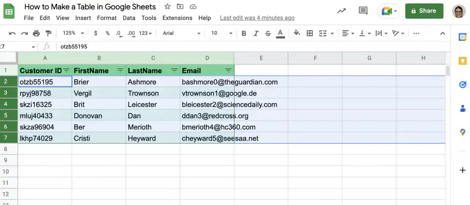
Collapsible table in Google Sheets — rows 2 to 7 selected below the header row

2. Right-click in the row number area to get the menu and click “View more row actions”. Select the option to group rows.

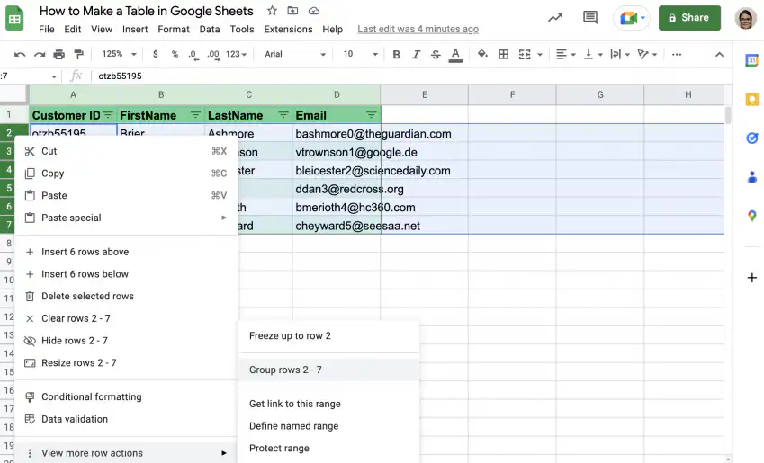
Collapsible table in Google Sheets — Group rows 2 - 7 under View more row actions

3. Click the minus symbol in the top-left corner to collapse the rows.

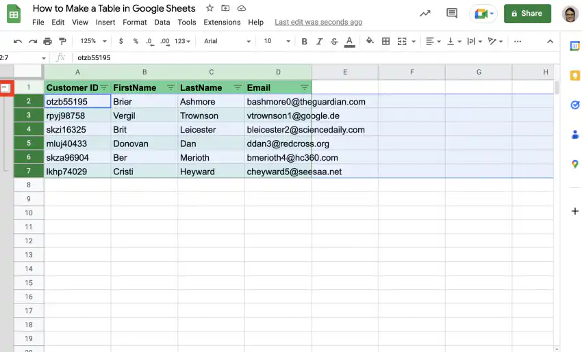
Collapsible table in Google Sheets — minus symbol to the left of the grouped rows

4. That’s it. To expand the table, simply click the plus symbol in the top-left corner.

Collapsible table in Google Sheets — rows collapsed under the header, with a plus symbol to expand them

Group table columns

Follow the steps below to group table columns so you can collapse and expand them as needed.

1. Select the columns you want to be able to collapse.

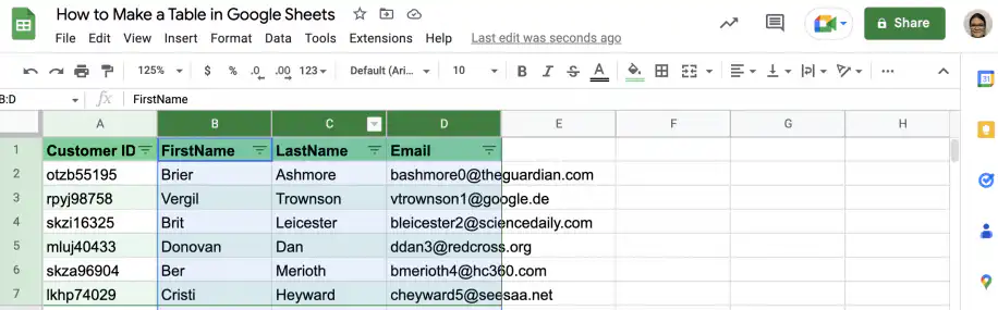
Collapsible table in Google Sheets — columns B to D selected

2. Right-click in the area with the column letters to get the menu, and click “View more column actions”. Select the option to group columns.

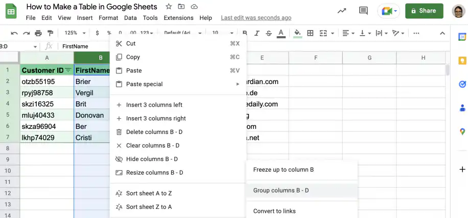
Collapsible table in Google Sheets — Group columns B - D under View more column actions

3. Click the minus symbol above the first grouped column.

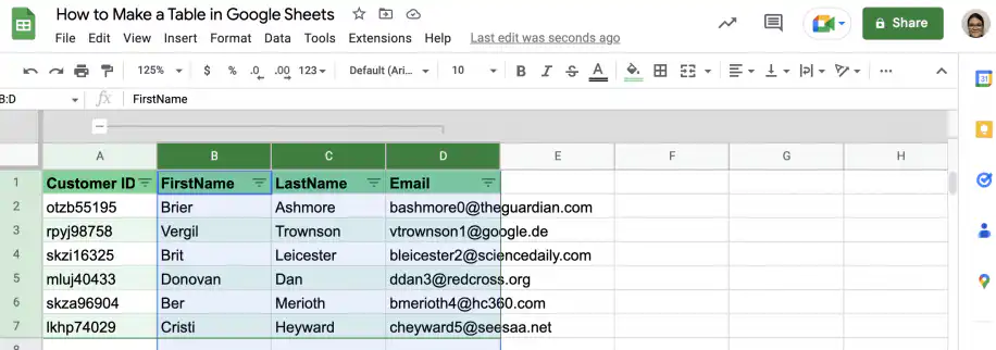
Collapsible table in Google Sheets — minus symbol above grouped columns B to D

4. That’s it. To expand the columns, click the plus symbol shown below.

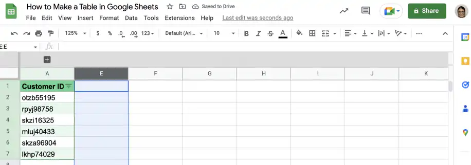
Collapsible table in Google Sheets — columns B to D collapsed, with a plus symbol above them

How to name a table in Google Sheets with named ranges?

If you frequently refer to data in your tables in other tables or formulas, named ranges will save you a lot of time. You can name the entire range, as well as individual columns. This allows you to search for and manipulate data by referring to the range name or the column name.

Below, you have step-by-step instructions on how to name your whole table, as well as specific columns within that table. Finally, you have an example of how to use a named range in a Google Sheets function.

1. Select the range of cells containing your table.

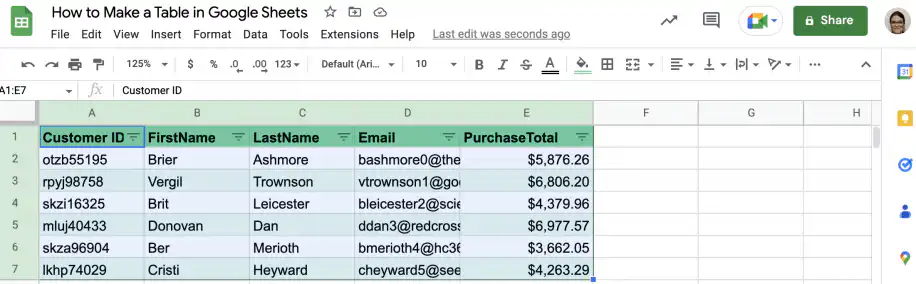
Name a table in Google Sheets — table range A1:E7 selected, with a PurchaseTotal column

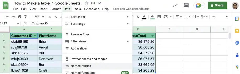
2. Go to Data > Named ranges.

Name a table in Google Sheets — Named ranges in the Data menu

3. Type in the name you want to use for your table and click “Done”.

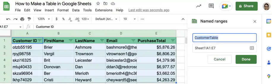
Name a table in Google Sheets — CustomerTable typed in the Named ranges sidebar for Sheet1!A1:E7

4. The table now appears in the “Named ranges” sidebar.

5. To name a column in your table, select the column and click “Add a range”.

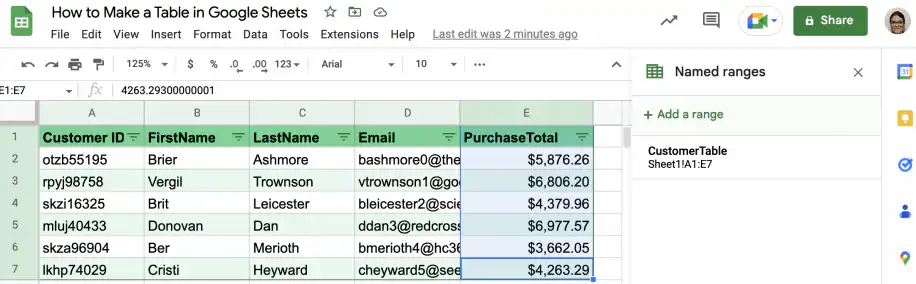
Name a table in Google Sheets — column E selected and Add a range in the Named ranges sidebar

6. Type a name for the column, such as PurchaseTotal, and click Done. Now that the column has a name, you can reference it from other cells, for example to find the total sum of purchases.

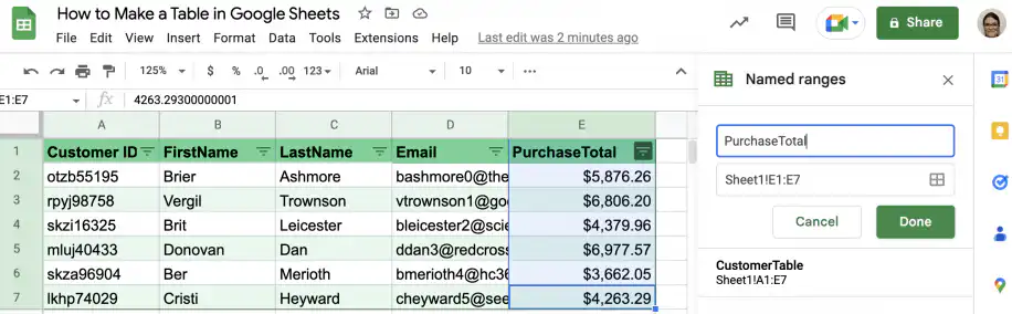
Name a table in Google Sheets — PurchaseTotal typed as the name for Sheet1!E1:E7

7. In an empty cell, type in the SUM function.

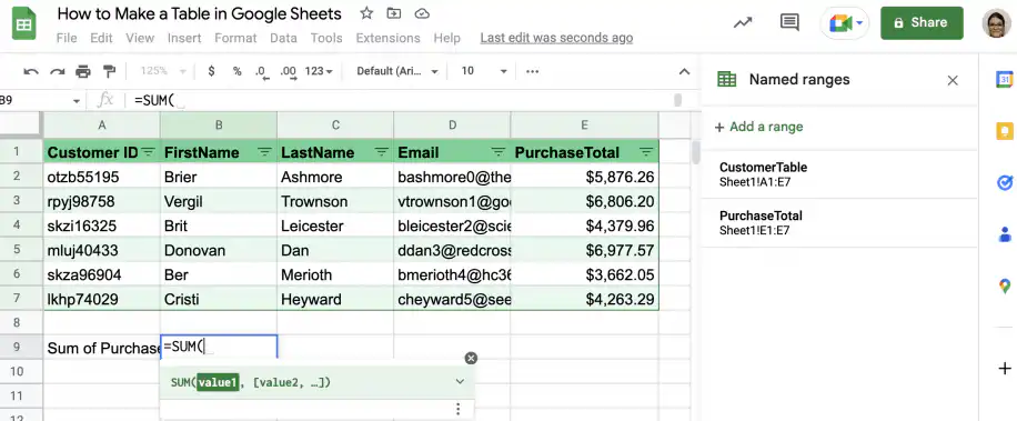
Google Sheets named range in a formula — =SUM( typed in B9 next to the Sum of Purchases label

8. After the parenthesis, start typing the name of the column. You will see a suggestion box like the one below. Click or hit the Tab key to select the column.

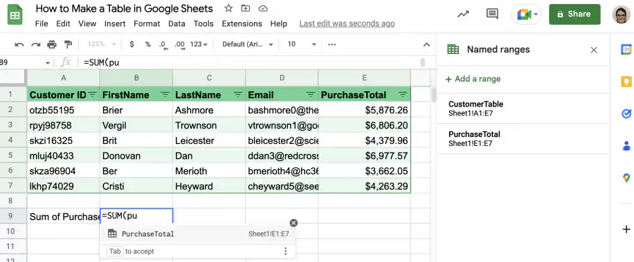
Google Sheets named range in a formula — PurchaseTotal suggested while typing =SUM(pu

9. Close the parenthesis and press ‘Enter’.

10. That’s it. You have the sum of all purchases.

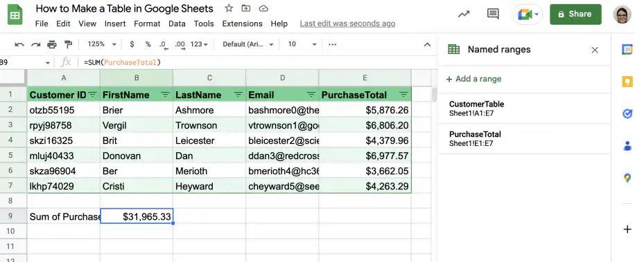
Google Sheets named range in a formula — =SUM(PurchaseTotal) returns $31,965.33

You can create a table in Google Sheets

And there you have it! This guide showed you five ways to create tables in Google Sheets. You can create and design the table manually or use AI (Gemini) to do it faster. You also saw how to group rows and columns so a long table can collapse, and how to give a table and its columns names you can use in formulas.

You can also check out the following guides to make better Google Sheets tables.