Google Sheets pivot tables: how to create and use them

A pivot table turns a long list of rows into a short summary you can read at a glance, such as total costs per department or the average price per neighborhood. You build it with a few clicks instead of formulas, and you can rearrange it whenever the question changes.

This guide shows how to create a Google Sheets pivot table step by step, how to edit and filter it, and how to turn it into a chart.

What are pivot tables?

Pivot tables are a powerful tool for extracting and analyzing the information you need from a large dataset. They’re an easy way to “slice and dice” data in spreadsheets: in other words, to filter and then group data. For example, you might want to examine sales for a specific year (slice) and then break it down by product category (dice).

The name comes from the way you can pivot the data, turning rows into columns and back, to look at the same numbers from another angle.

The significant advantage of pivot tables is that they are dynamic, quicker, and more reliable than manually typing formulas.

Pivot tables enable different users to customize the structure and design of tables, allowing them to view the specific data they need. Within the same organization, each stakeholder is interested in different aspects of operations. Even within departments, coworkers use slightly different KPIs or filters to achieve the same goal.

If you’ve used Excel, you’re probably already familiar with Pivot tables, and Google Sheets has the same tool.

What can pivot tables in Google Sheets be used for?

If your work involves finding key patterns, trends, or making a comparative analysis on large datasets, pivot tables in Google Sheets help in these ways:

Easier interpretation: By summarizing data, pivot tables help users focus on key information and get a better understanding of the information they present.
Faster pattern and trend spotting: This can be achieved through sorting and rearranging data according to the type of information you seek.
Reliable decision-making: Rows and columns can be rearranged to compare data in a more straightforward way. This will also improve decision-making for managers since they gain a holistic view of their data.

Now that you’ve seen the most useful ways to use pivot tables in Google Sheets, let’s see how you can easily create them.

How to create a pivot table in Google Sheets

Making a pivot table in Google Sheets takes five steps.

Step 1: Select the data source

Open a new spreadsheet in Google Sheets and click File > Open
Select a file from Google Drive or upload a new file in any spreadsheet format.

In this example, I’m using publicly available data from Airbnb listings in Paris. This dataset has listed rooms and apartments in Paris, including indicators such as neighborhood, room type and price.

Step 2: Select the data range of the pivot table

Select all of the cells containing data.
In this case, I will select all columns to be included in the pivot table (a shortcut is to use Ctrl+A). Now I will customize and edit the variables/KPIs I want to include.

Note: your columns must have a named header in the top row to use the data in the pivot table.

Step 3: Insert the pivot table

Go to Insert in the menu bar and select Pivot table.
For a better overview, we will add the table to a new sheet. Click Create.
A new sheet called “Pivot Table 1” opens. On the right-hand side you see the pivot table editor.

How to create a pivot table in Google Sheets — Create pivot table dialog with New sheet selected

Step 4: Pivot table editor

Google is smart so it automatically provides suggestions for how to analyze your data set.
In this example, the second suggestion is what we want to see: Airbnb listings in Paris by room type.

Step 5: Customize the pivot table

I want my pivot table to show the average prices for each neighborhood in Paris. This is where pivot tables are really useful: they let you analyze information quickly without writing formulas.

In the pivot table editor, under Rows, click Add and choose “neighborhood” from the listings spreadsheet.

Under Values, click Add, then select price.

Click Summarize by dropdown and select Average.

Select Column B (price) and change the format to currency.

Google Sheets pivot table — average price per Paris neighbourhood with the pivot table editor open

Let’s extract more data. Suppose I want to know how many days of the year these rooms are available.

Go to Values, click Add and select availability_365.

Summarize by AVERAGE.

Google Sheets pivot table — average price and availability per Paris neighbourhood

That’s it: these are the basic steps for creating a pivot table in Google Sheets.

In this example, I’ve created a pivot table that shows the average price for a room in each neighborhood of Paris and the number of days per year these rooms are available.

From a huge data set containing more than 60,000 Airbnb listings, I can easily reach various insights:

Average price of accommodation in Paris is €118.
Average availability per accommodation is 80 days per year.
There is a price deviation in the Élysée neighborhood where a room costs €247 on average.

How to add a pivot table to an existing sheet

The steps above put the pivot table on a new sheet. To add it next to your data instead:

1. Go to Insert > Pivot table and check the data range.

2. Under Insert to, choose Existing sheet, then click the grid icon in the field below it.

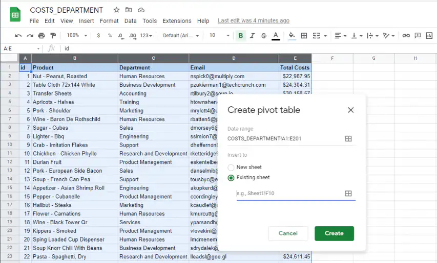
Google Sheets pivot table — Create pivot table dialog with Existing sheet selected

3. Click the cell where the pivot table should start, or type its reference, and click OK. Then click Create.

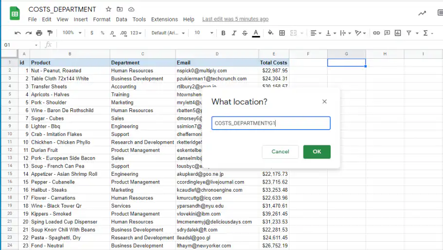
Add a pivot table to an existing sheet — What location box set to cell G1

Pick a spot with empty space below it and to its right, because the pivot table grows as you add fields.

How to create a pivot table from Google’s suggestions

For a quick summary, let Google Sheets build the pivot table for you. Suggestions won’t cover advanced needs, but they take seconds.

1. Insert an empty pivot table as shown above.

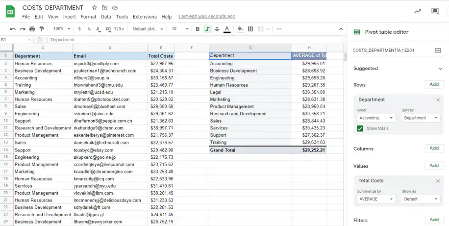
2. In the pivot table editor, open Suggested and pick one. Here, it’s “Average of Total Costs for each Department”.

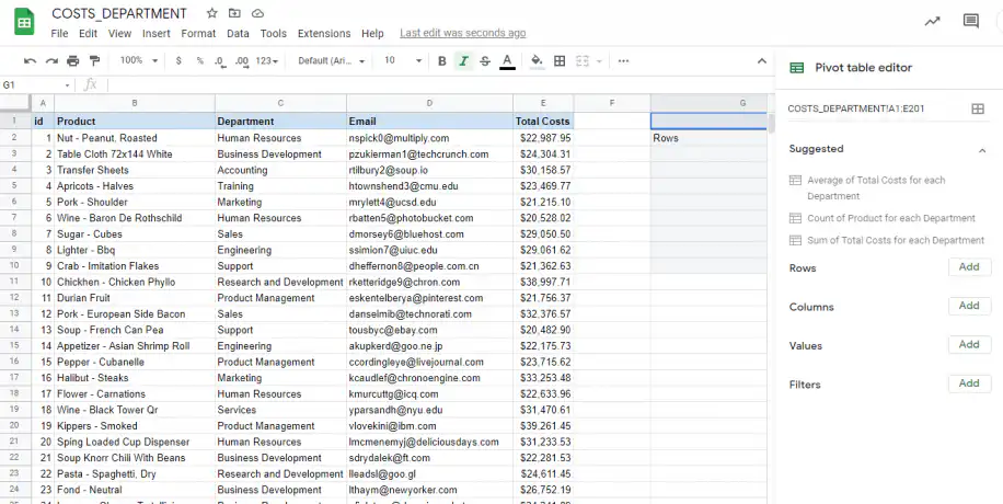
Google Sheets pivot table suggestions — Suggested list in the pivot table editor

3. The pivot table fills in right away, and you can still edit it like any other.

Google Sheets pivot table suggestions — average of Total Costs for each department

How to edit a pivot table in Google Sheets

Add a filter to the pivot table

You have already filtered your data by creating a pivot table, but you might want to break that information down into further categories. You can do that by adding an extra filter in the pivot table editor.

Go to Filter. Again, Google Sheets provides automatic suggestions based on your data.

If you want to add a different filter, click Add. Next to Showing all items, click the ⏷dropdown menu.

You can:

Filter by condition (e.g. text contains). You can then enter a value, a cell reference or a field.
Filter by value.

Note: if you apply a filter and then update your source data, you need to update your pivot table filter.

Looking at the Airbnb data, let’s say I want to analyze my data by room type. First I add a column for room type. But I only want to see results for: hotel room, private room and shared room. Under Filter I select those rooms.

Edit a pivot table in Google Sheets — Airbnb prices by neighbourhood split into room type columns

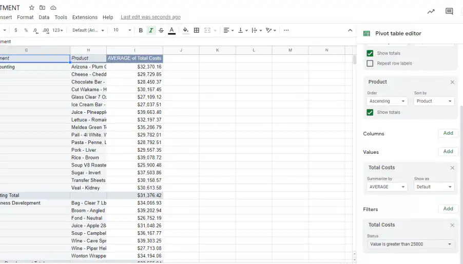
Filter by condition is the quickest way to focus on the biggest numbers. In this second example, a table of costs per department, Total Costs is under Filters. Open Showing all items and choose Filter by condition.

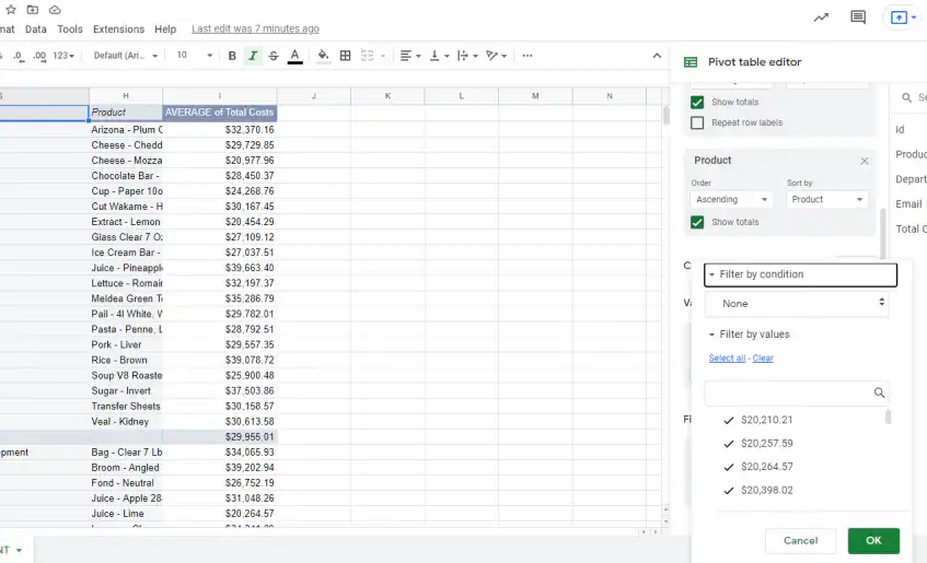
Filter a Google Sheets pivot table — Filter by condition option in the Total Costs filter

Pick Greater than and enter the threshold, here 25,000. The pivot table now lists only the items above it.

Filter a Google Sheets pivot table — Total Costs filter set to value is greater than 25000

How to sort and summarize pivot table data

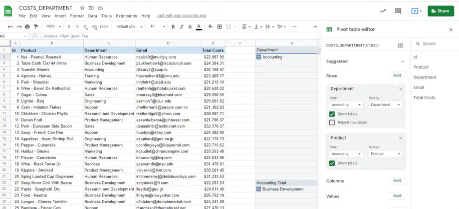
Each field under Rows or Columns has its own Order and Sort by settings. In this example, the rows show Department and then Product, both in ascending order. Switch Order to Descending, or sort by a value such as SUM of Total Costs, to put the biggest numbers first.

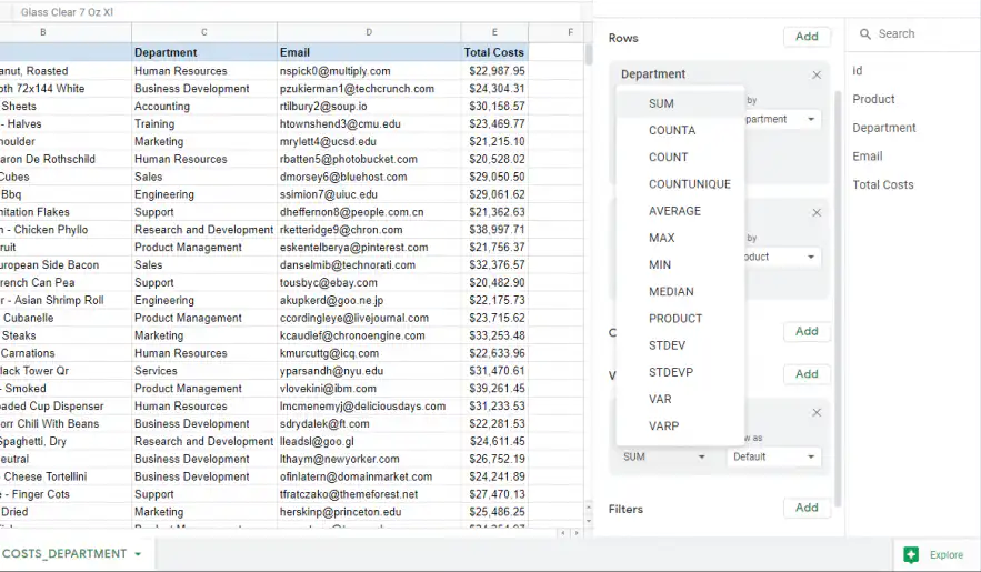
Sort a Google Sheets pivot table — Department and Product rows with Order and Sort by settings

Under Values, Summarize by sets the calculation, such as SUM, COUNT, AVERAGE, MAX, or MEDIAN. Show as displays each result as is or as a percentage of its row, its column, or the grand total.

Summarize a Google Sheets pivot table — Summarize by list with SUM, COUNT, AVERAGE, MAX, and MIN

How to group rows in a pivot table

To combine several row items into one group, select them in the pivot table, right-click, and choose Create pivot group. For a date column, right-click a date and choose Create pivot date group, then pick a period such as Month or Year. To undo a group, right-click it and choose Ungroup pivot items.

How to customize rows and columns

If Google’s automatic suggestions don’t match what data you need, you can adjust the Rows, Columns, Values, and Filter manually.

Deselect Google’s default suggestions by clicking X, then Add, and selecting which row or column you want to pull data from.

You can change the header names by clicking directly on a row or column.

Add a custom formula

In the pivot table editor on the right-hand side, go to Values > Add > Calculated field.

Enter your formula, then go to Summarize by, and click Custom. A new column appears called “Calculated field 1.”

For help with writing formulas in Google Sheets, see Google’s full function list here.

How to create a pivot chart in Google Sheets

Google Sheets has no separate pivot chart tool. You add a regular chart on top of the pivot table, and the chart follows the pivot table when you change it.

1. Click any cell inside the pivot table.

2. Go to Insert > Chart. Google Sheets picks a chart type and uses the pivot table as the data range.

3. In the chart editor, open the Setup tab and choose a type under Chart type. A column or bar chart compares totals per category. A pie chart shows how each category adds up to the whole.

4. Open the Customize tab to change the chart title, axis titles, and colors.

If you add a filter or switch Summarize by from SUM to AVERAGE, the chart updates with the pivot table. When the pivot table gains rows outside the chart’s data range, extend the range in the Setup tab. And if the Grand Total shows up as its own bar, untick Show totals for that row field in the pivot table editor.

For more chart options, see how to insert a chart in Google Sheets or how to make a pie chart in Google Sheets.

How to make a pivot table from multiple sheets

A pivot table reads one data range. If your data sits on another tab of the same file, type that tab’s range in the Data range field, for example Sales!A1:E500. If it’s split across several tabs or files, combine it into one range first:

Copy and paste the data into one table. That works for a one-off report, but the copy goes stale as soon as the sources change.
Use formulas. QUERY can stack tabs on top of each other, and IMPORTRANGE pulls data in from another file.
Use Sheetgo, an AI-powered data automation platform, to combine Google Sheets from several files into one sheet on a schedule, so the pivot table always reads current data.

Then build the pivot table on the combined range, as shown above.

That’s how to do a pivot table in Google Sheets

You’ve now got an overview of how to create a pivot table in Google Sheets. Pivot tables have many uses and they can get quite complicated, hopefully this post helped you get started.

Looking for other quick ways to filter data in your spreadsheets? Check out our post on sorting and filtering data in Google Sheets.

Working in Excel too? See how to create a pivot table in Excel.