


The SPARKLINE function in Google Sheets draws a small line, bar, column, or win/loss chart inside a single cell.
Syntax: =SPARKLINE(data, [options])
| Option | What it sets |
|---|---|
| charttype | "line" (the default), "bar", "column", or "winloss" |
| color | Line or column color, as a name or a hex code. Bar charts use color1 and color2. |
| max | The value that fills the whole cell in a bar chart |
| ymin, ymax | The bottom and top of the scale in line and column charts |
| empty | How to treat empty cells: "zero" or "ignore" |
| nan | How to treat cells that aren’t numbers: "convert" or "ignore" |
Example: =SPARKLINE(C2:F2,{"charttype","column";"color","green"}) draws a green column for each value in C2:F2.
If you want a quick way to analyze your spreadsheet data visually without building full charts, the SPARKLINE function in Google Sheets is a great solution. It allows you to create mini charts inside individual cells, so you can quickly visualize trends.
Take a look at the example below. Imagine I’m a teacher and I want to analyze my students’ test scores:

As you can see, the results don’t exactly jump out at you from a sea of numbers. And when the data extends further across the spreadsheet, it becomes increasingly difficult to see how your students are doing over time. If I have 100 students who have all taken 15 tests, there’s no way I can analyze the trends with my bare eyes.
It isn’t feasible, time-wise, to build a chart for every single student, but that’s where SPARKLINE function in Google Sheets comes to the rescue. The function allows you to create a mini sparkline chart in a single cell. There are four main types:
- Line sparkline — this is the default sparkline in Google Sheets
- Column sparkline — like a mini column chart in one cell
- Bar sparkline — a mini bar chart in one cell
- Winloss sparkline — a mini column chart for yes/no or positive/negative results


Syntax
- data – this is the reference to the range of cells that you want to plot as a sparkline
- options – these are used to customize the chart. Google has a full list here. These can be applied in two ways:
- As an array of option key and option value pairs, following the data parameter.
- As an address reference to a two column range, where the first column cells hold the option keys, and the second column cells hold the corresponding option values.
How to insert a sparkline in Google Sheets
- Click the cell where the chart should go, usually next to the row of data.
- Type =SPARKLINE( and select the data range, for example C2:F2.
- To change the chart, type a comma and add options in curly brackets, such as {"charttype","column"}. A comma separates an option from its value, and a semicolon separates one option from the next.
- Close the parenthesis and press Enter. To add a sparkline to every row, drag the fill handle down.
The chart resizes with its cell, so widen the column or make the row taller if you want a bigger sparkline.
How to use SPARKLINE function
SPARKLINE(data_range)
To accommodate the sparklines, I will insert a blank column after the Name column and give it a header name ‘Trend’. Now, in cell B2, I’ll type in the function =SPARKLINE(C2:F2):

Hit the Enter key, and the Sparkline appears in cell B2. As a result, the miniature version of a chart is nicely embedded within the area of the cell.

To create a sparkline for every student, drag the formula all the way down (or copy and paste it):

These sparklines make it much easier to read large datasets quickly. In this example, I can spot upward or downward trends for my students much more quickly than analyzing each student’s scores individually.
SPARKLINE(data_range, color_option as key value pair)
Next I’ll show you how to change the color of the lines in the sparkline. Notice that both the key (“color”) and value (“red”) are within double quotes, and that they are within curly braces/brackets that indicate an array of key value pairs:

The formula here is =Sparkline(C2:F2,{"color","red"}).
SPARKLINE(data_range, [color_option and line_thickness as key value pairs])
If the lines are too thin, you can simply increase the width. To do that you need to include an additional option key-value pair, as shown below. Notice that the two key-value pairs are separated by a semi-colon.

The formula here is =Sparkline(C2:F2,{"color","red";"linewidth",3}).
SPARKLINE(data_range, [column chart_type, other color_options as key value pairs])
What if you don’t want line graphs at all? You can change the sparkline to other types of chart. Here I’ll try a column chart and different colors. As you can see, it’s probably not the most attractive or readable sparkline, but it gives you an idea of what you can do.

You can also use Hex codes to indicate the colors, like this:


Win/Loss SPARKLINE
At this point you’ve seen examples of both the line and column types of sparklines. What about the win/loss chart type? This is useful for binary data – items that are either ‘yes’ or ‘no’, 1 or 0, heads or tails, etc.
In the example below, I’ve changed the data to a binary value of 1 (if the student passed the test) or 0 (if they failed). By using the win/loss format, you can quickly analyze this type of data.

Barchart for quick data visualization
In this example, I’ll show how to use the bar chart sparkline type to quickly visualize data in a simple way. This is a basic example, but a great way to put simple one-dimensional data into an easy-to-view format.

This is done by typing =Sparkline(B2,{"charttype","bar";"max",100}).
Chart options referenced in other cells
In this example, instead of hardcoding the chart options into the formula, I’ll put the options into a table that will be referenced in the function. This allows for easy changing of the options. It’s especially useful if you want to play around with different options to see what looks best.

SPARKLINE examples by chart type
Each chart type below comes with a formula you can copy. Change the range and the options to fit your data.
Line sparkline
Line charts are most useful for displaying data that changes over consistent time intervals. For example, =SPARKLINE(A2:D2,{"charttype","line";"color","indigo";"linewidth",2}) draws a thicker indigo line across the four values in A2:D2. If you leave out charttype, you still get a line, because line is the default.
Bar sparkline
A bar sparkline draws a horizontal bar from a single value. It works well when you compare every cell in a column: put =SPARKLINE(A13,{"charttype","bar";"max",100}) next to the first value and fill it down. Set the max option, or each bar fills the whole cell.
Column sparkline
If you’re interested in comparing a series of values against each other, use the SPARKLINE function to draw a column chart, like the one below. Column sparklines can show negative values in a color of their own.
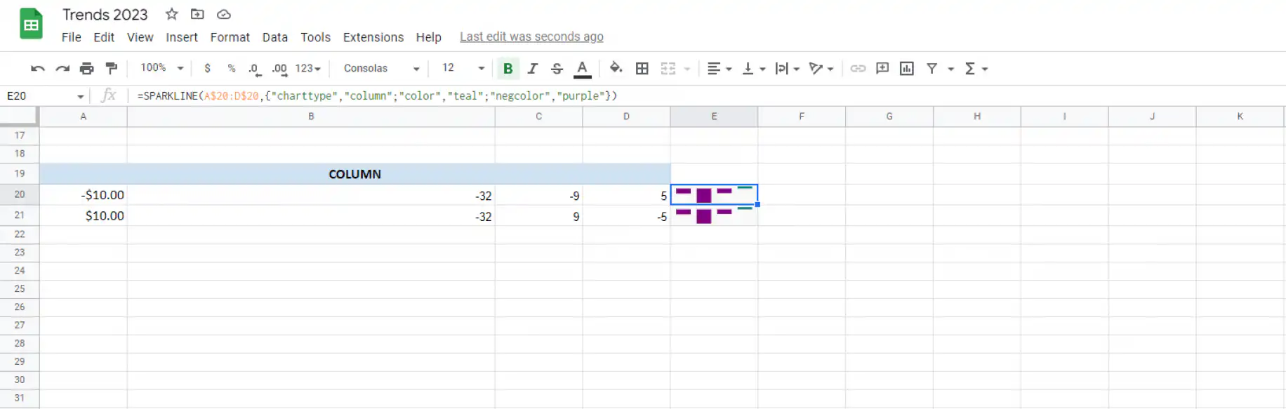
The formula in the screenshot is =SPARKLINE(A$20:D$20,{"charttype","column";"color","teal";"negcolor","purple"}). Positive values show as teal columns and negative values as purple ones.
Vertical bar sparkline
SPARKLINE has no vertical bar chart type. The bar type always draws horizontal bars, so for vertical bars, use the column type shown above. Each value in the range becomes one vertical bar.
Win/loss sparkline
The win-loss chart type allows you to display binary data, such as wins and losses. You can also use colors to highlight specific data in more ways.
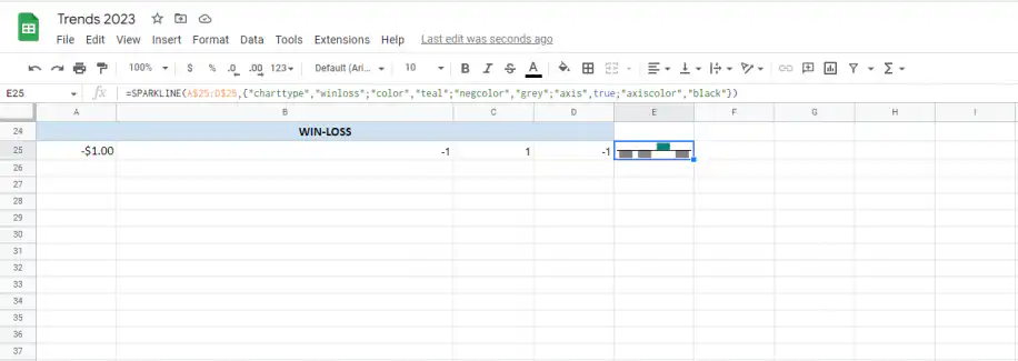
Here the formula is =SPARKLINE(A$25:D$25,{"charttype","winloss";"color","teal";"negcolor","grey";"axis",true;"axiscolor","black"}). Every value above zero gets a teal bar above the axis, and every value below zero gets a grey bar below it. The axis option draws the black line between them.
That’s it, that’s how you use the SPARKLINE function in Google Sheets. It has a ton of customization options and it’s a really handy visualization tool to make your spreadsheets more user-friendly and make the data easier to read.
Want to know how to insert charts in Google Sheets or make larger charts with your data however? Read our blog posts on how do I insert a chart in Google Sheets and how to create a dashboard in Google Sheets.
For a full-size chart instead of a sparkline, see how to create a bar chart in Google Sheets or how to create a trendline in Google Sheets.
If the numbers behind your sparklines come from several spreadsheets, Sheetgo, an AI-powered data automation platform, can bring them into one sheet on a schedule, so your charts stay current without copy and paste. See how to automate reports using dashboards.
Editor’s note: This is a revised version of a previous post that has been updated for accuracy and comprehensiveness.

 English
 Español
 Português do Brasil
 Français