




The internal rate of return (IRR) is a concept in financial modeling commonly used in combination with net present value (NPV). The formula in Excel is used to estimate the rate of return an investment would give based on a series of cash flows, usually presented as a percentage (‘3%’). The NPV, on the other hand, is expressed as a cardinal number (‘3’). Both play a key role in making investment decisions when presented with more than one opportunity, as we will show here.
This article will provide step-by-step guidance on how to use the IRR formula to effectively calculate the IRR for investment decisions. If you work in Google Sheets instead, see how to use the IRR formula in Google Sheets.
How to use the IRR function in Excel?
We will first explain how to use the IRR function in Excel to calculate the rate of annual return for an initial investment. If you need to calculate return rates for different time periods or a future value, Excel also offers a variety of financial functions, such as XIRR or MIRR.
What is the formula for calculating IRR?
The syntax for the IRR formula is:
=IRR(values,[guess])
- values: This argument is required. It refers to the cash flows, the initial investment (as a negative figure), and net income (as a positive figure).
IMPORTANT: It is important that the initial investment and cash flows maintain the same sequence, as the IRR formula will interpret them in this very order. Moreover, for the IRR function to work properly, the argument should be a number. If it is a logical value, text, or an empty cell, it will be ignored.
- [guess]: This argument is optional. It is an estimation of the number closest to the expected IRR (as there can be two). If not included, the argument will show the default value of 0.1 (=10%).
Let’s now apply the IRR formula, to the following scenario:
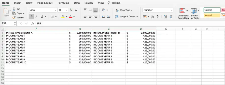
You are a business owner and you are presented with two investment opportunities, A and B. The first has an initial investment of $2,500,000.00, whereas the second has one of $2,800,000.00. The net income for each is presented on a yearly basis. The IRR function can help you get an idea of what the return rate would be based on the initial investment and the yearly cash inflows:
1. Option A has an initial investment of $2,500,000.00 with the following yearly cash flows.
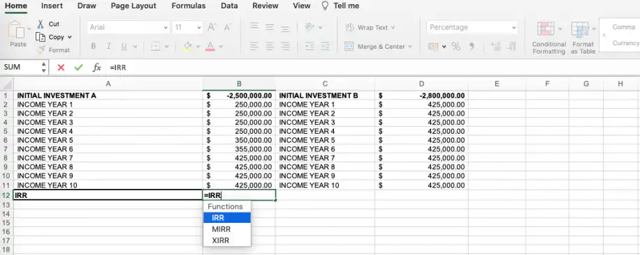
2. Type in ‘IRR’ in the cell you wish to showcase the IRR value.
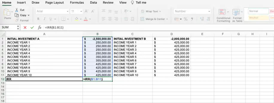
3. As soon as you select from the drop-down menu, you will automatically be prompted to select the cell range that you wish to perform the IRR calculation on.
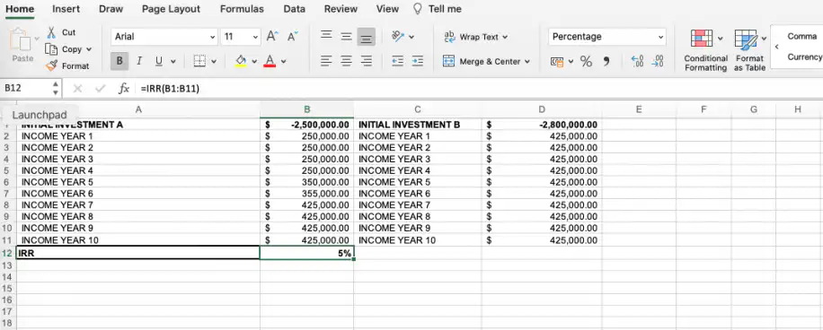
4. Once you press the Return key you will be shown the IRR percentage. Remember that IRR is represented as a percentage, whereas NPV is a cardinal number. Here, we get a return of 5%.
5. Now, let’s calculate the IRR for Option B with an initial investment of $2,800,000.00 and the following yearly cash flows.
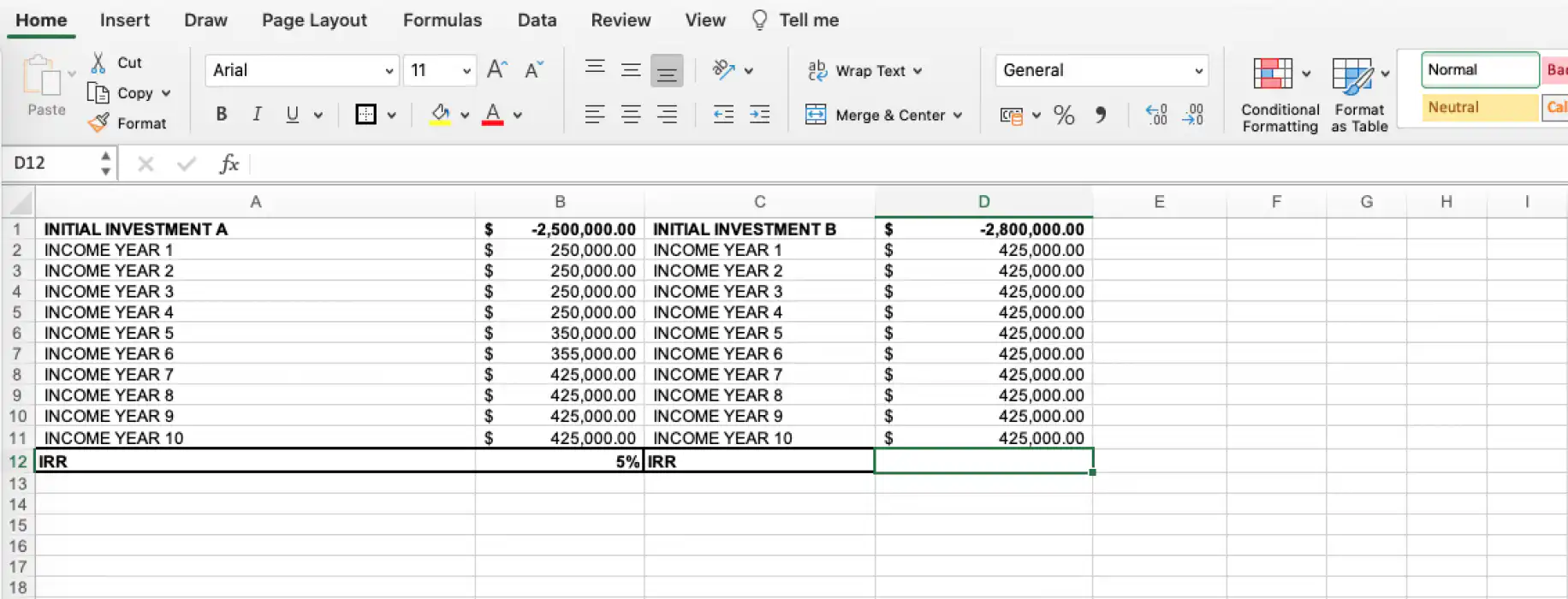
6. We would input the formula in the same way we did previously in steps 2-3.
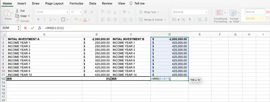
7. Here, we get an IRR of 8%.
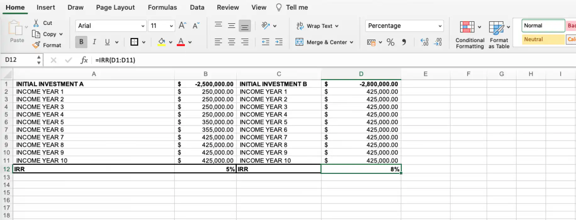
The information obtained so far would help us decide solely based on the IRR; it is common practice to go for the higher percentage. Considering that Option A provides an IRR of 5% and B of 8%, we would opt for investing in project B. However, if the cash flows were on a monthly basis, our decision-making could be more precise. By following these steps, you can easily learn how to calculate IRR in Excel for monthly cash flow.
How to calculate IRR using NPV in Excel?
As mentioned in the Introduction, the NPV is expressed as a cardinal number, as opposed to the IRR which is expressed as a percentage. It is used to calculate the difference between current cash inflow and outflow over a period of time. Make note that the “rate” referred to in the NPV formula is not the same as the rate obtained using the IRR formula shown previously:
- rate: refers to the discount rate for the investment period. This discount rate is a generic term used to refer to any rate that is established, subjectively or objectively, to discount future cash flows with. Moreover, for more reliable decision-making, we should always apply a lower and a higher discount rate for all investment options.
- values: refer to the initial investment (represented as a negative value) and the cash inflows over the given time periods.
Let’s say that we apply a 5% discount rate (this could represent the lower rate) to both investment opportunities.
1. Type in ‘NPV’ in the cell you want to obtain the NPV formula.
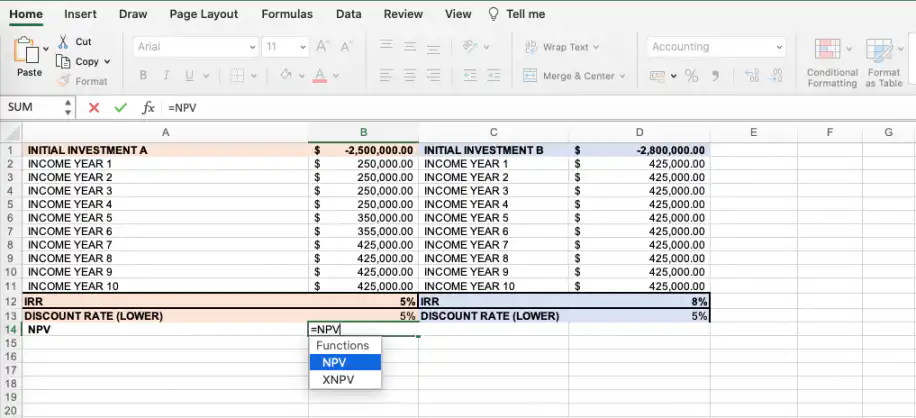
2. As the first parameter corresponds to the discount rate, we first need to add cell B13 followed by the sum of cash flows, and finally add all to the initial investment.
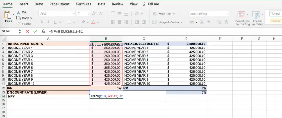
3. Press the Return key to obtain the NPV value ($50,196.47).
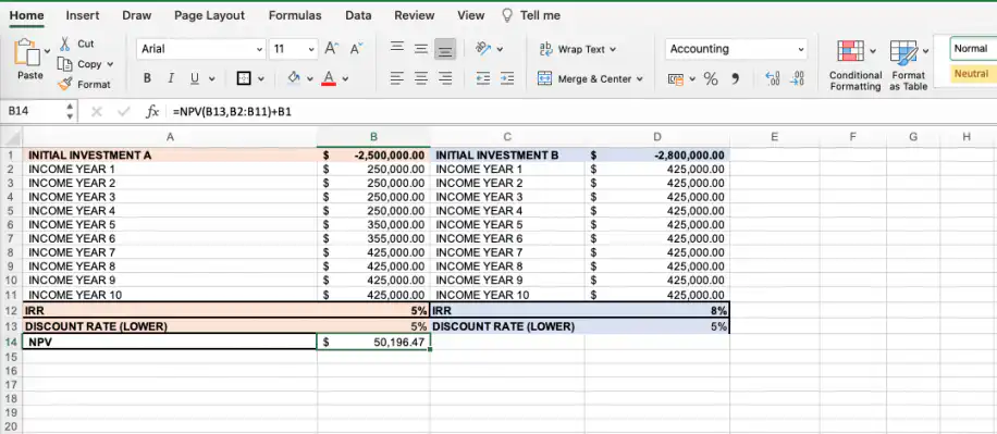
4. To calculate the NPV for investment option B, follow steps 1-3.
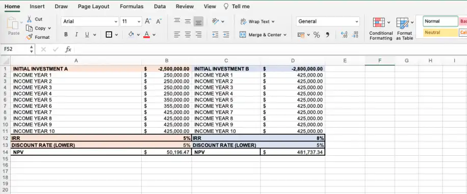
As mentioned before, we would now need to calculate the NPV for a higher discount rate (8%) for both investment opportunities. Once again, let’s start with option A.
5. We have included a second row where we will calculate the NPV applied to the same values as before, but this time include cell B15 as the discount rate.
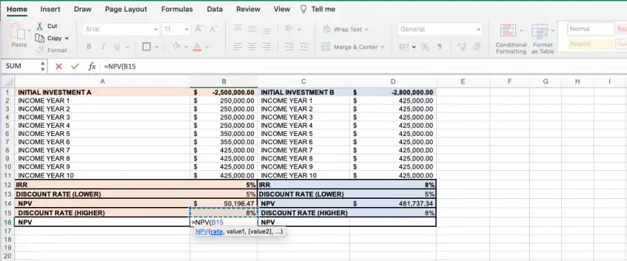
6. Proceed to apply values to the NPV formula and press the “return” key to obtain the result:
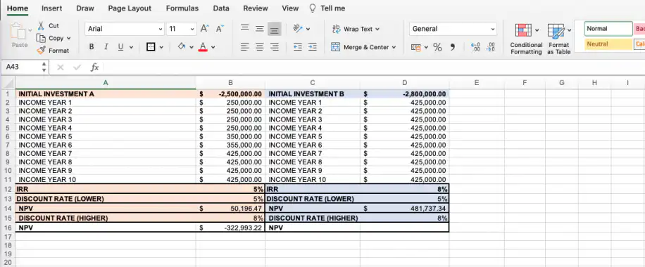
7. For investment option B, we have followed steps 5 and 6 and obtained the following:
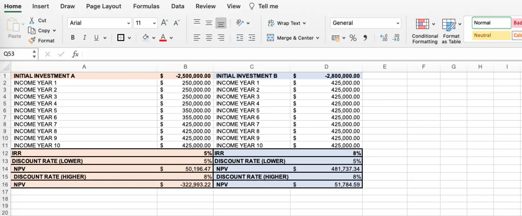
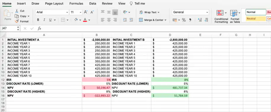
Based on the obtained results, we decide on Option B. Why? Because both the NPV and IRR are higher in both discount rate scenarios:
The IRR formula can only be used in instances where the cash flow distribution occurs over the same time periods (yearly, monthly, etc.). If you want to calculate the rate of return for different time periods, use the XIRR formula in Excel. This selects the cash flow range and then the range of dates on which the cash flows are made.
How do you calculate IRR manually?
If you are advanced in math or aren’t interested in calculating IRR in Excel, this is what you would need to do to calculate IRR manually:
1. Estimate two discount rate values (i.e., 4% and 8%) to try and set the NPV to zero.
2. Calculate the NPVs using 4% and 8% and try to get as close to zero as you can.
3. Once you determine your two discount rate values and the two NPVs, you can use this formula to calculate the IRR:
IRR = R1 + ( (NPV1 * (R2 - R1)) / (NPV1 - NPV2) )
4. R1 corresponds to the lower discount rate (4%) and R2 is the higher one (8%). NPV1, on the other hand, represents the higher NPV, and NPV2 the lower.
Conclusion
This article has explained the concepts of IRR and NPV, followed by a step-by-step process showing how to calculate IRR in Excel, how to use the IRR function in Excel in combination with NPV function, and finally broken down the use of IRR by explaining how to calculate IRR manually.
Whether you wish to explore further on financial functions or apply the functions seen in this post to real-time investments, you will find the article on How to use the GOOGLEFINANCE Function in Google Sheets very useful.
To run the same check in Google Sheets, read how to use the NPV formula in Google Sheets. For a full valuation built on discounted cash flows, start from our DCF template in Google Sheets. If your cash flow figures live in several spreadsheets, Sheetgo’s AI finance virtual employee can pull them into one up-to-date file.



 English
 Español
 Português do Brasil
 Français