Combine QUERY with IMPORTRANGE in Google Sheets

Combining QUERY with IMPORTRANGE allows you to pull in data from different spreadsheets and perform advanced queries on it. Whether you’re managing project progress, financial data, or team efforts, mastering these functions can enhance your productivity and data management.

IMPORTRANGE is one of the most useful Google Sheets functions. As the name suggests, it imports a range of cells from one spreadsheet to another.

On the other hand, QUERY is an incredibly versatile formula, essentially allowing you to use your spreadsheet as a database. With SQL-like query language, you can look up, sum, count, average, filter and sort data.

Below you’ll find the syntax, five examples, and a step-by-step setup in two real files, including how to allow access and how to group and sort the imported data.

How to use QUERY with IMPORTRANGE in Google Sheets

This combination applies QUERY directly to the data transferred with IMPORTRANGE to filter specific columns, rows, and ranges.

It’s a real time-saver when working with multiple spreadsheets, as you only pull in the exact data you need. It also allows you to format the data within your query instead of afterwards, which saves you an additional step.

Syntax

• spreadsheet_url – the link to the spreadsheet where data is imported from.
• range_string – range of cells to be imported. This can be further broken down into two components: 
  • sheet_name – the name of the sheet with the desired data 
  • cell_range – the range of the cells within this sheet
• query – criteria of which data to transfer. Query handles language functions (Select, Group by, etc.) and data manipulation functions (Avg, Sum, Count, and Multiply).

How does this combination work?

Whenever you combine functions, things can get a bit confusing. To avoid that, let’s look at what’s going on in this syntax.

First, let’s focus on QUERY. This function can manipulate data in many ways, but always needs to start with a data source.

In many cases this is data from another tab on the same spreadsheet. But as you know, this article deals with importing data from another spreadsheet. As a result, we will use the IMPORTRANGE function to feed data into QUERY.

IMPORTRANGE is a simple function: just input the link to the spreadsheet and the range you want to import. The first time you connect two files, it shows a #REF! error until you allow access. The step-by-step setup further down shows where to click.

This imported data can be plugged into the QUERY function. After all you need to input are the query parameters, which dictate how the data will be manipulated and displayed. The examples below illustrate this.

Just remember, the structure of the syntax remains similar, no matter which function you nest inside Google Sheets’ QUERY function.

Example 1: Import and Query

In the following examples, I’ll use this geographical data as the source data:

First, I import country data from 186 countries into a business spreadsheet. I’ve merged items from a separate dataset based on certain criteria.

Say I only want to import the data from countries in the Americas. To display only those specific cells, you simply need to apply the Select and Where clauses inside the QUERY function.

In this formula, QUERY searches data from a predefined range/array according to specific criteria. Simultaneously, IMPORTRANGE imports the data into the target spreadsheet.

Placing QUERY before IMPORTRANGE allows you to search (query) specific information from the data that is imported with IMPORTRANGE. This way, you only import the data you want to see in your spreadsheet.

After IMPORTRANGE, you need to add search criteria. To import data from countries in the Americas, we used this query: Select * Where Col1=’Americas’.  In plain English that translates to “select all the data that has “Americas” in column 1”.

This formula comes in especially  handy in situations where you want to merge data. If you work in online marketing for example, you might want traffic from various sources into one spreadsheet. It gives you a better overview of several data sources such as Google Analytics, Ahrefs, SEMrush or Google Search Console.

Example 2: Import data within a date range

In this next example, I added search criteria after IMPORTRANGE. In this case, where Col3 > date ‘2019-07-01’ and Col3 < date ‘2019-12-30’ imports the same data but only for items in the list that were published between those dates.

Note that when you input a date into your query, you need to type the word date before it. Also don’t forget to put the date in quotation marks. That’s how the function knows you’re referring to a date.

You might apply this formula in logistics or even for a small business cash register. You can add up rows, columns and data ranges with changes in the data over time. If you’re interested in changes to product lines, sales, and other KPIs over the course of the year, this formula can carry out monthly or quarterly comparative analysis.

Example 3: Import and combine multiple spreadsheets with specific criteria

If you want to extract certain cells or a range from several spreadsheets, use the following formula. Here’s how to merge data from multiple spreadsheets into one:

You need to use IMPORTRANGE for every spreadsheet you want to merge. Within the first IMPORTRANGE formula, I added the headers in A1:P.

The other spreadsheets also contain the headers. However, they should not be imported multiple times. To avoid importing the header three times, I’ve changed the range to A2:P on the second and third sheets.

Lastly, the Where clause (where Col1<>’’) simply states that all cells that are not blank should be imported.

Here are a few tips for importing multiple sheets:

• The list of imports needs to be enclosed in curly brackets and a semicolon must separate each IMPORTRANGE.
• The imported sheets must all have the same layout. For example, if the first column of all the sheets wasn’t Country Name, the data wouldn’t combine properly.
• Don’t import the headers on every sheet – you only need one.
• Remember to allow access to all the spreadsheets you want to import from.

This formula is really useful for business surveys (when you collect several spreadsheets with the same format). Likewise for educational purposes. When you hand out similar exercises to students or when you collect grades from various professors.

Example 4: Import and Query Average Values

With this formula, I import the average population of each continent. As you can see, I add “avg” after the ‘Select’ clause and I put the column in parentheses. Next, add the query (the data you are looking for) after the Where clause. In this case, the query is ‘Europe’.

Notice how on the rest of this spreadsheet I use multiple QUERY/IMPORTRANGE functions to get average populations and total GDPs for different regions. Since QUERY is highly customizable, you can get all sorts of different outputs depending on your objective!

QUERY function allows you to extract all arithmetic functions. This is a very helpful tool for traders and financial analysts. With it, you can look up values from a variety of investment spreadsheets and carry out calculations such as Present Value =PV, Future Value =FV and interest rate functions such as =IRR and =RATE.

In addition: it’s a more intuitive, natural language version of the complex INDEX-MATCH formulas in Excel.

Example 5: Import and Query Sum values

In this final example, the formula filters by continent, sums up each country’s GDP and imports data from a separate spreadsheet.

This is specifically helpful to create dashboards and reports of all kinds.

How to set up QUERY with IMPORTRANGE between two files

The examples above use a placeholder for the spreadsheet URL. Here is the whole setup in a real pair of files, with the URL and the range in their own cells so the formula stays short.

The example below is based on two files. The source file contains data on sales for all agents and products. The destination file is where I want to import and analyze data based on specific conditions.

Copy the source URL and cell range

1. Open both the source and destination files in Sheets.

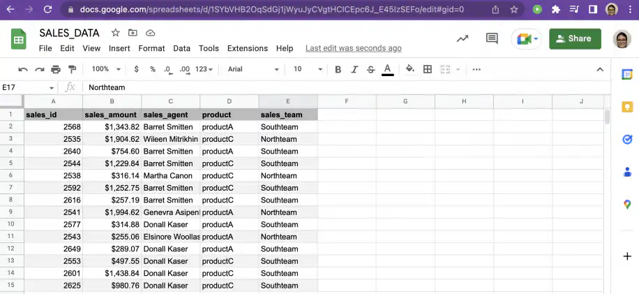
2. From the source file, copy the URL.

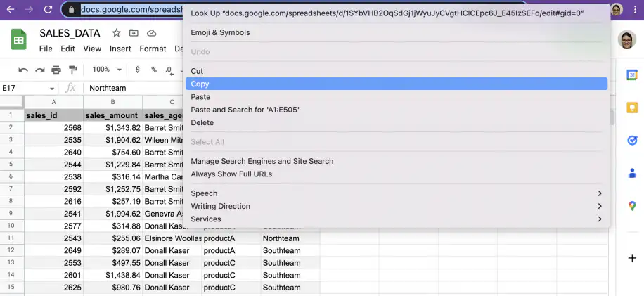
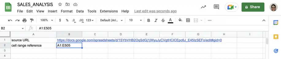
3. Paste the URL into the destination file.

4. Go back to the source file and select the cell range. You can copy the cell range reference from the top-left corner, as shown below.

5. Paste the cell range reference into the destination file. I don’t need to specify the sheet because it is on “Sheet1”.

Add the QUERY function

I’ll use a simple query with ‘select’ and ‘where’ clauses to import the rows where the “sales_team” is the ‘Southteam’.

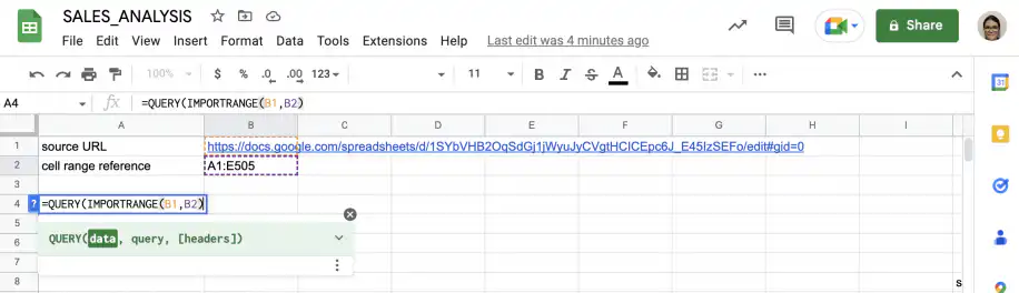
1. Start typing the formula for QUERY.

2. For the ‘data’ argument, add IMPORTRANGE and reference the cells that hold its arguments, B1 and B2.

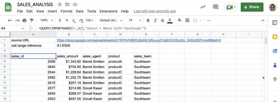
3. For the ‘query’ argument, I will use “Select * Where Col5=’Southteam'”. ‘Col5’ is the column “sales_team”, which should match the “Southteam”.

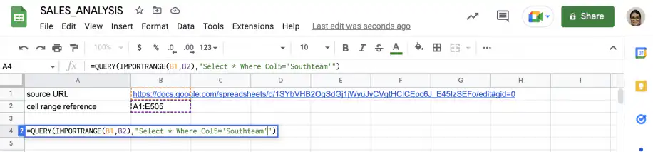
4. Press “Enter” to see the results.

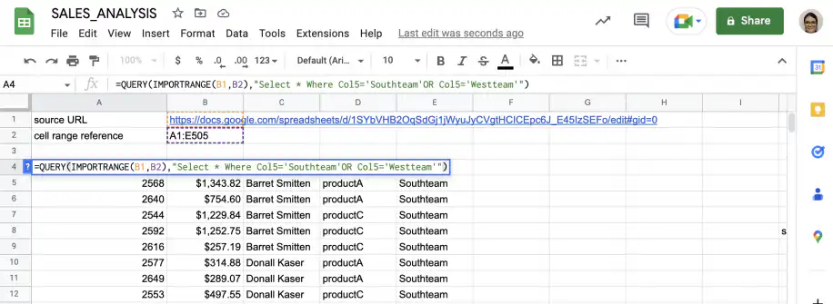
5. You can easily add another condition by using the ‘OR’ operator. For instance, I can import the results for two different teams by adjusting the query as shown below.

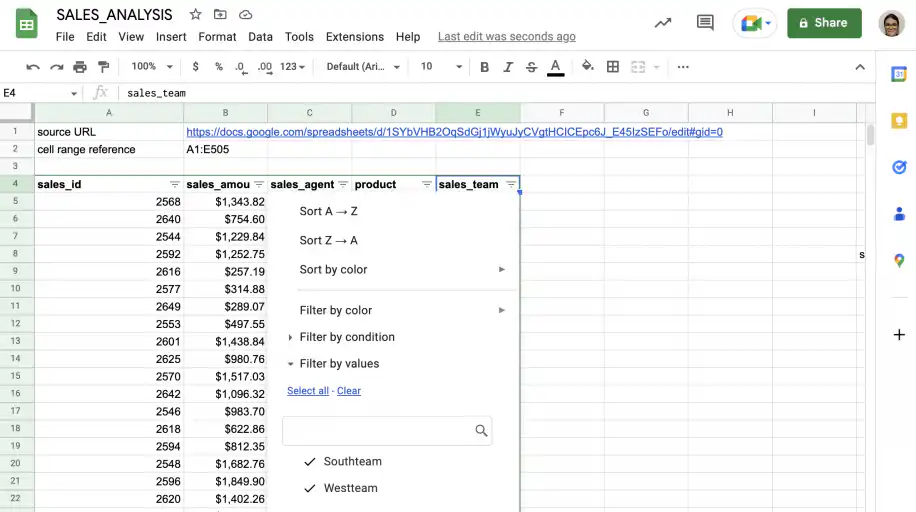
6. As you can see in the screenshot below, the results now also contain the data for ‘Westteam’.

Allow access between the files

If you’re working with files that have never been connected before, you’ll see an error message instead of the value when you press ‘Enter’. To see the actual value, you will have to approve access between sheets. Click the cell with the #REF! error, then click Allow access. You only need to do this once for each pair of files.

How to group and sort imported data with QUERY

For the sake of simplicity, I’ll use the data from the previous section. For my analysis, I want to see sales totals by team, as well as sales totals by sales agent.

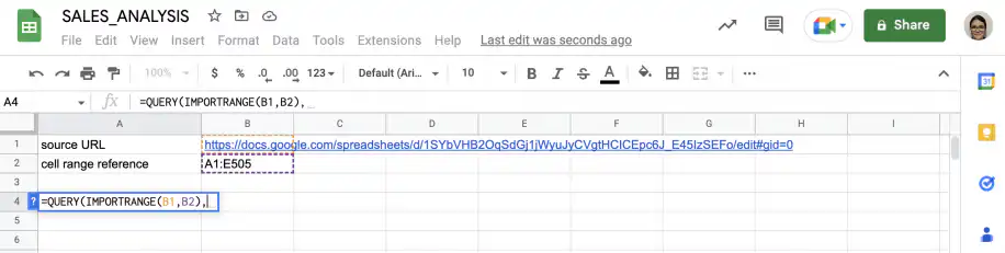
Group by sales team

To group the results, I need to select the ‘sales_team’ column (5) and the sum of the ‘sales_amount’ column, then group by ‘sales_team’.

The query looks like this: “Select Col5,sum(Col2) Group by Col5”.

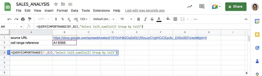
Press ‘Enter’ to see the results.

Group by sales agent

As the name of the sales agent is in column 3, I need to modify the query and replace references to ‘Col5’ with ‘Col3’.

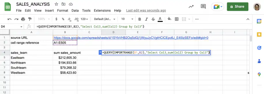
Press ‘Enter’ to see the results.

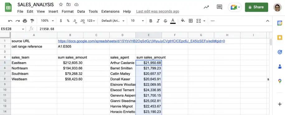
Order by sales amount

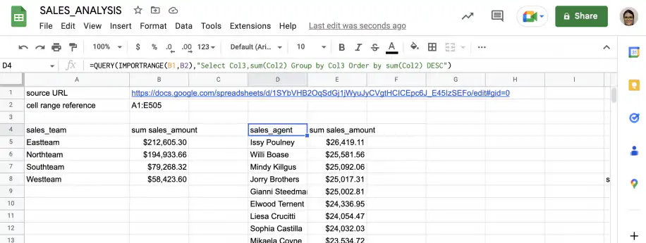
As you can see in the previous screenshot, the function automatically sorts the column alphabetically by the name of the sales agent. However, I want to see the results by sales amount, in descending order.

I can modify the previous query by adding “Order by sum(Col2) DESC” at the end.

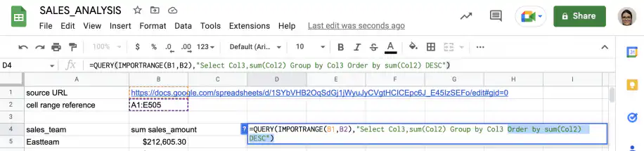
Press ‘Enter’ to see your results ordered by sales amount.

Get the same results with Sheetgo connections

Sheetgo offers an intuitive and powerful alternative to the combination of QUERY and IMPORTRANGE in Google Sheets. With Sheetgo, you can import and process data automatically, so your spreadsheet data is ready for reports, dashboards, and AI.

Coincidentally, one of the key data processing capabilities of Sheetgo offers QUERY filter. This feature enables you to perform advanced data queries similar to the QUERY function in Google Sheets. You can filter, sort, and manipulate data as it flows between your spreadsheets, all without the need for complex formulas.

Why use Sheetgo over IMPORTRANGE? Here are just three reasons:

• Enhanced Data Management: Unlike IMPORTRANGE, Sheetgo provides a centralized dashboard where you can manage all your data connections.
• Scalability: Sheetgo can handle large datasets and multiple connections without the performance issues that IMPORTRANGE might encounter. This makes it ideal for businesses with complex data requirements.
• Advanced Filtering: With Sheetgo’s QUERY filter, you can perform sophisticated data manipulations directly within your workflows. This allows for more advanced data processing capabilities compared to IMPORTRANGE.

Find out all the reasons why Sheetgo is the best IMPORTRANGE alternative.

Conclusion

Now you’ve got the lowdown on how to use QUERY with IMPORTRANGE, from allowing access between files to grouping and sorting the imported data. Now you can merge the power of these two functions, for another great combination check out How to use VLOOKUP and IMPORTRANGE.

If your dataset is too large for QUERY+IMPORTRANGE to handle, the no-formula IMPORTRANGE alternative shows how to filter and connect Google Sheets at scale without crashing.