Get help

Help center

Guides and answers

Contact support

Write to our team

Sign in to

Workflows

Build processes with your team

Automations

Connect files and automate tasks

One system, four parts

AI agents

Virtual Employees that work 24/7

Automations

Connect files and automate tasks

Workflows

Build processes with your team

Data Space

Trusted data sharing and control

Solutions by department

Finance

Reports, budgets, and reconciliations

Inventory and manufacturing

Stock, orders, and production in one view

HR

Timesheets, attendance, and reviews

Project management

Status and workload across projects

Sales and CRM

Leads and deals kept up to date

Education

Student records and school data

Finance

Turn manual finance work into reports that update themselves.

What Finance teams automate

  • Track payables and receivables
  • Build cash flow statements
  • Compare budget against actuals

Inventory and manufacturing

See stock levels and automate ordering.

What inventory and manufacturing teams automate

  • Track inventory across multiple sites
  • Connect sales, purchasing, and warehouse data
  • Link a barcode scanner to your sheet

HR

Run recruitment, attendance, and OKR tracking from your sheets.

What HR teams automate

  • Track recruitment and onboarding
  • Record team OKRs and results
  • Track check-ins, check-outs, and leave

Project management

Assign tasks and track hours without manual updates.

What project teams automate

  • Assign tasks and track status changes
  • Estimate effort and log hours worked
  • Track milestones across projects

Sales and CRM

Track leads and sales performance with automated reports.

What sales teams automate

  • Track and convert leads
  • Set sales goals and track team metrics
  • Monitor sales KPIs on dashboards

Education

Automate attendance, grades, and school purchasing.

What schools automate

  • Track attendance and notify parents
  • Record and compare class grades
  • Track inventory lent to students and staff

Find a use case

By department

How each team uses Sheetgo

By industry

How each industry uses Sheetgo

By company size

Small, medium-sized, or large

Learn

Blog

Guides and product news

Customer stories

How teams like yours use Sheetgo

Help center

Guides and answers

Why Sheetgo

Compare

How Sheetgo compares with other tools

Security

How we protect your data

Trust center

Our compliance details

Sign in to

Workflows

Build processes with your team

Automations

Connect files and automate tasks

One system, four parts

AI agents

Virtual Employees that work 24/7

Automations

Connect files and automate tasks

Workflows

Build processes with your team

Data Space

Trusted data sharing and control

Solutions by department

Finance

Reports, budgets, and reconciliations

Inventory and manufacturing

Stock, orders, and production in one view

HR

Timesheets, attendance, and reviews

Project management

Status and workload across projects

Sales and CRM

Leads and deals kept up to date

Education

Student records and school data

Find a use case

By department

How each team uses Sheetgo

By industry

How each industry uses Sheetgo

By company size

Small, medium-sized, or large

Get started

Templates

Ready-made workflows to start from

Learn

Blog

Guides and product news

Customer stories

How teams like yours use Sheetgo

Help center

Guides and answers

Why Sheetgo

Compare

How Sheetgo compares with other tools

Security

How we protect your data

Trust center

Our compliance details

Help center

Guides and answers

Contact support

Write to our team

Workflows

Build processes with your team

Automations

Connect files and automate tasks

How to make a pie chart in Google Sheets

A pie chart shows how the parts of a whole compare. Each slice is one category, and its size is that category’s share of the total, which makes it a good fit for a handful of categories such as the items in a monthly budget.

This guide shows you how to make a pie chart in Google Sheets, step by step. You’ll start with a basic chart, then turn it into a 3D or doughnut chart, show percentages or labels, change slice colors, add a title, and edit the chart when your data changes.

Insert a pie chart from your data range

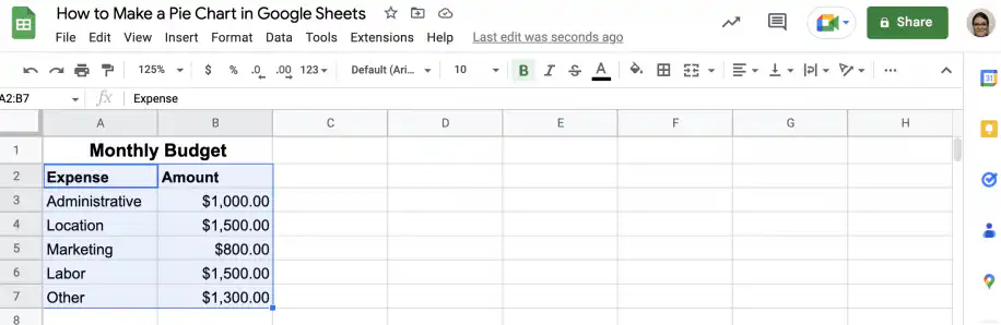
First, let’s create a simple pie chart based on a monthly budget. The table below contains the expense names and amounts used for the pie chart.

1. Open the Google Sheets file with the data.
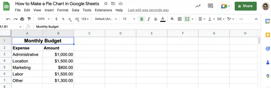
Pie chart in Google Sheets — monthly budget table with expense names and amounts

2. Select the columns with the data.

Make a pie chart in Google Sheets — expense and amount columns selected

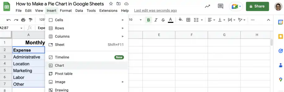
3. Go to Insert > Chart.

Make a pie chart in Google Sheets — Chart option in the Insert menu

4. That’s it. Google Sheets recognized the type of data and automatically inserted a pie chart. If it picks a different chart, double-click the chart, open the Setup tab in the Chart editor, and choose Pie chart under Chart type.
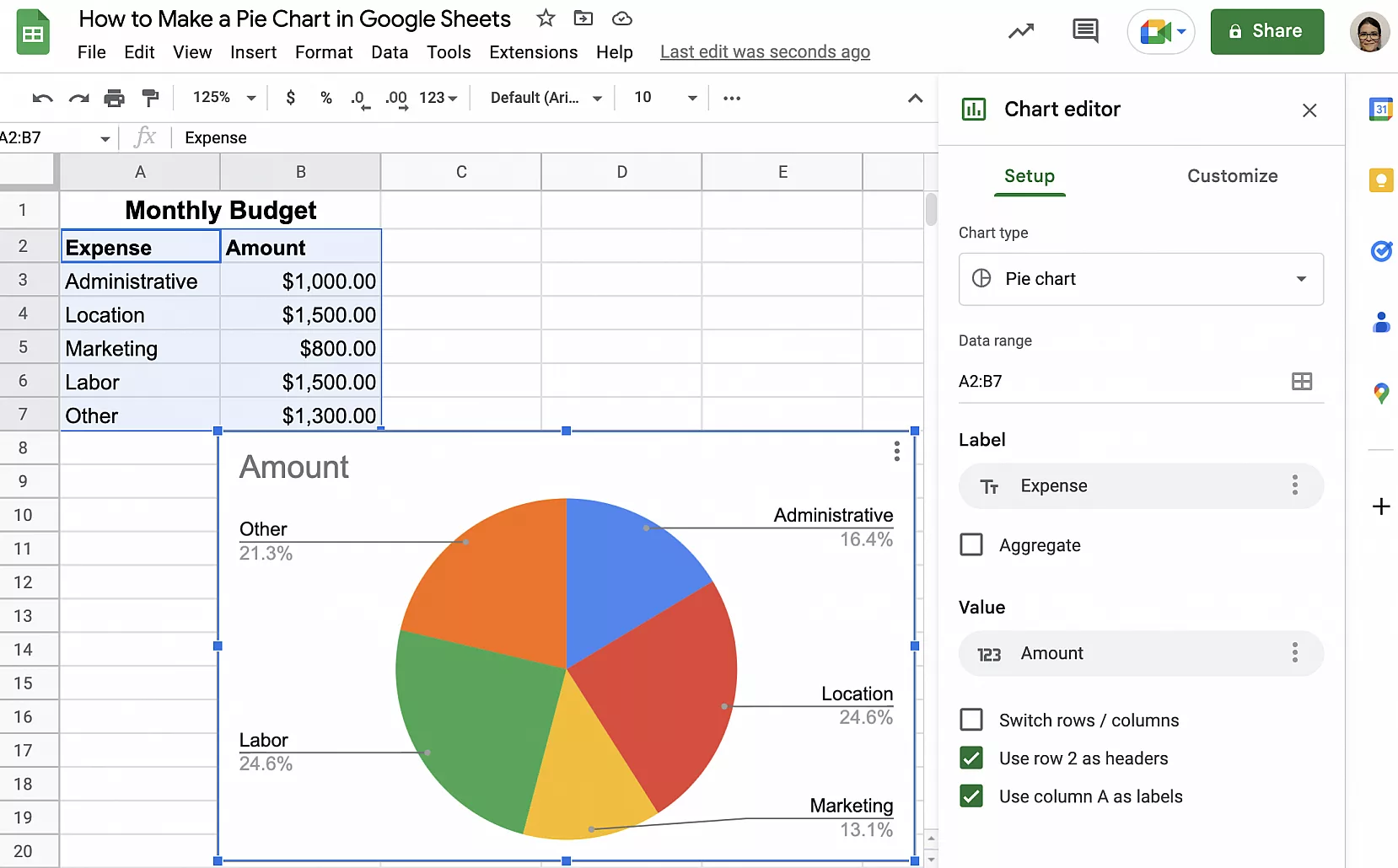
Google Sheets pie chart — budget pie chart with the Chart editor open on Setup

How to customize a Google Sheets pie chart

Now that you have a basic pie chart, let’s see how you can customize it to suit your needs and preferences. Follow the instructions below to change your pie chart to a 3D pie chart or a doughnut chart, display the percentages without labels, or change how the labels appear.

Make a 3D pie chart

Double-click your current pie chart to get the ‘Chart editor’ sidebar.

1. Click the ‘Customize’ tab in the ‘Chart editor’.
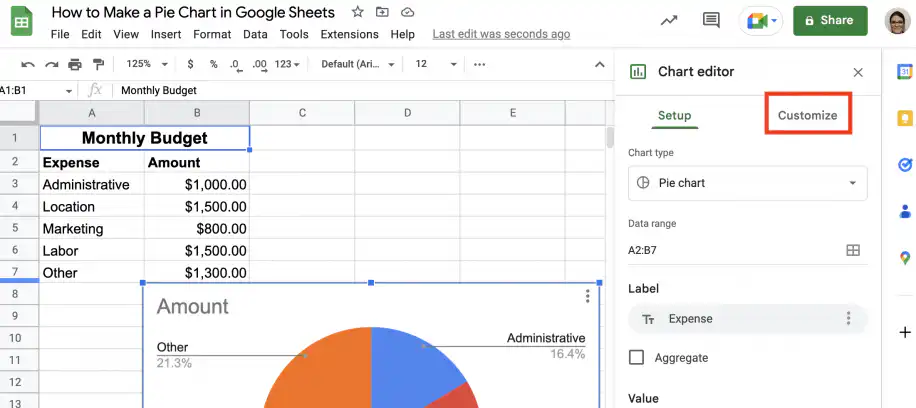
3D pie chart in Google Sheets — Customize tab in the Chart editor

2. Click ‘Chart style’ to expand the options.
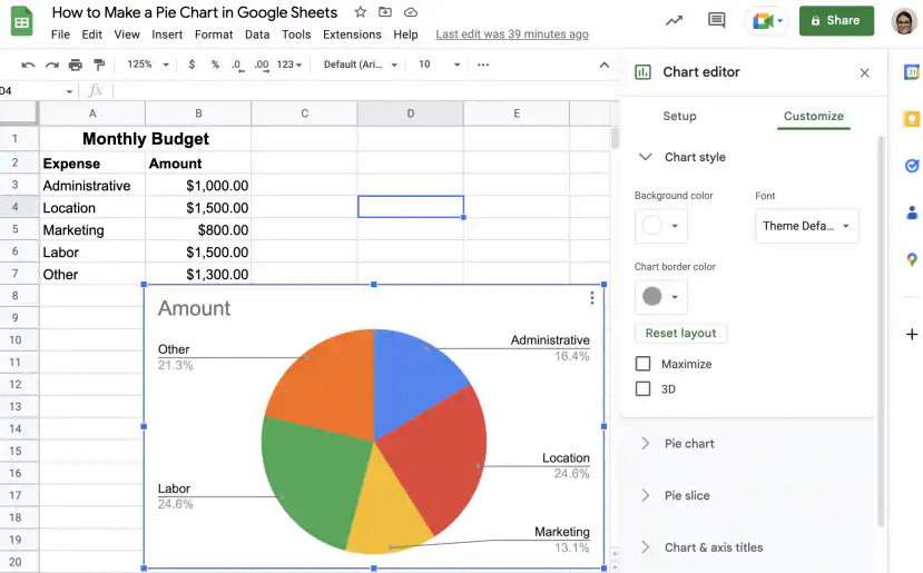
3D pie chart in Google Sheets — Chart style options with the 3D checkbox

3. Check the “3D” checkbox to turn it into a 3D pie chart.
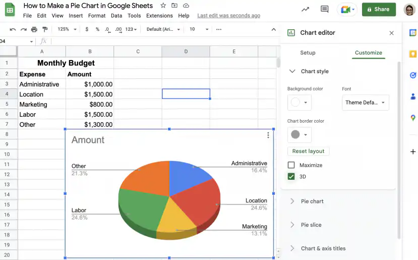
3D pie chart in Google Sheets — 3D checkbox ticked and the chart drawn in 3D

4. Alternatively, you can change it under ‘Chart type’ in the ‘Setup’ tab.
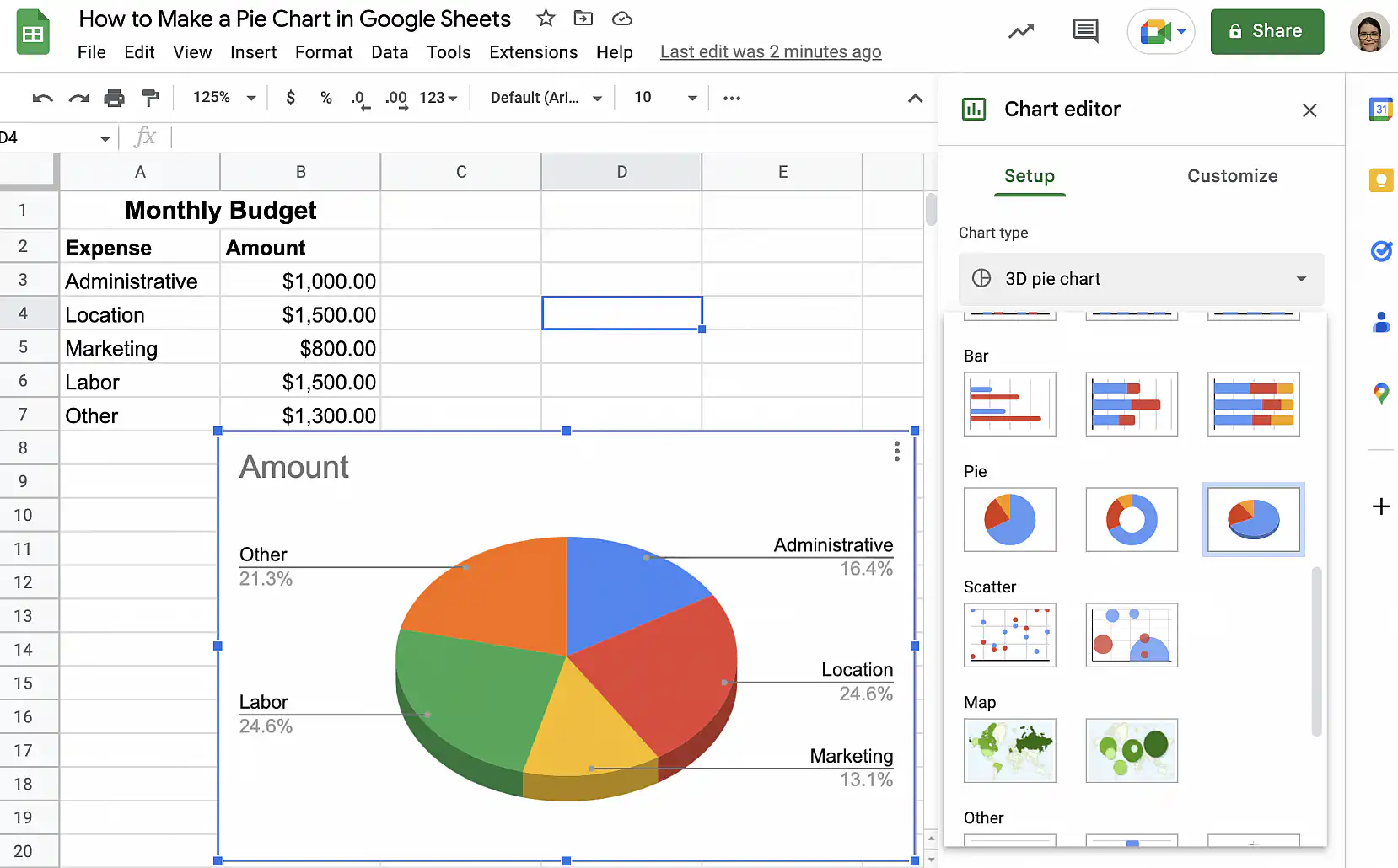
3D pie chart in Google Sheets — 3D pie chart picked under Chart type

Make a doughnut chart

If you prefer, you can quickly turn your pie chart into a doughnut chart.

1. Double-click your pie chart to get the ‘Chart editor’ sidebar. In the ‘Setup’ tab, click the drop-down under ‘Chart type’.
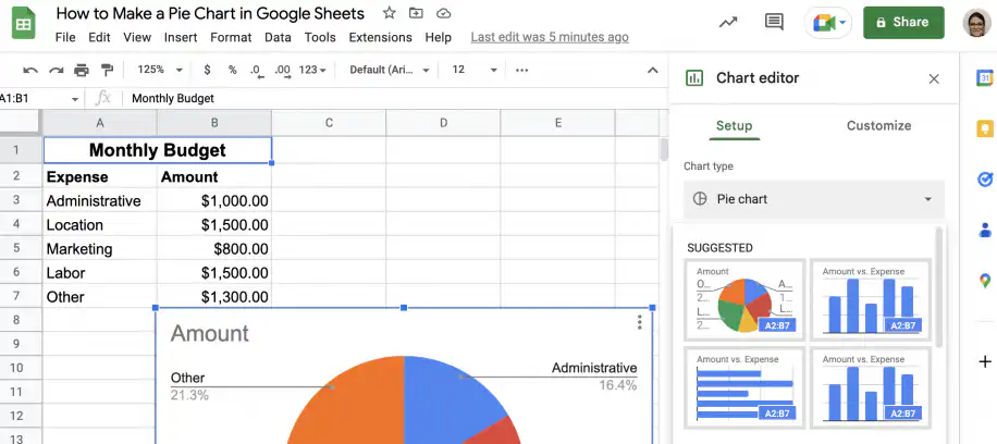
Doughnut chart in Google Sheets — Chart type drop-down menu open in the Setup tab

2. Scroll down to the ‘Pie’ area and select the doughnut chart.
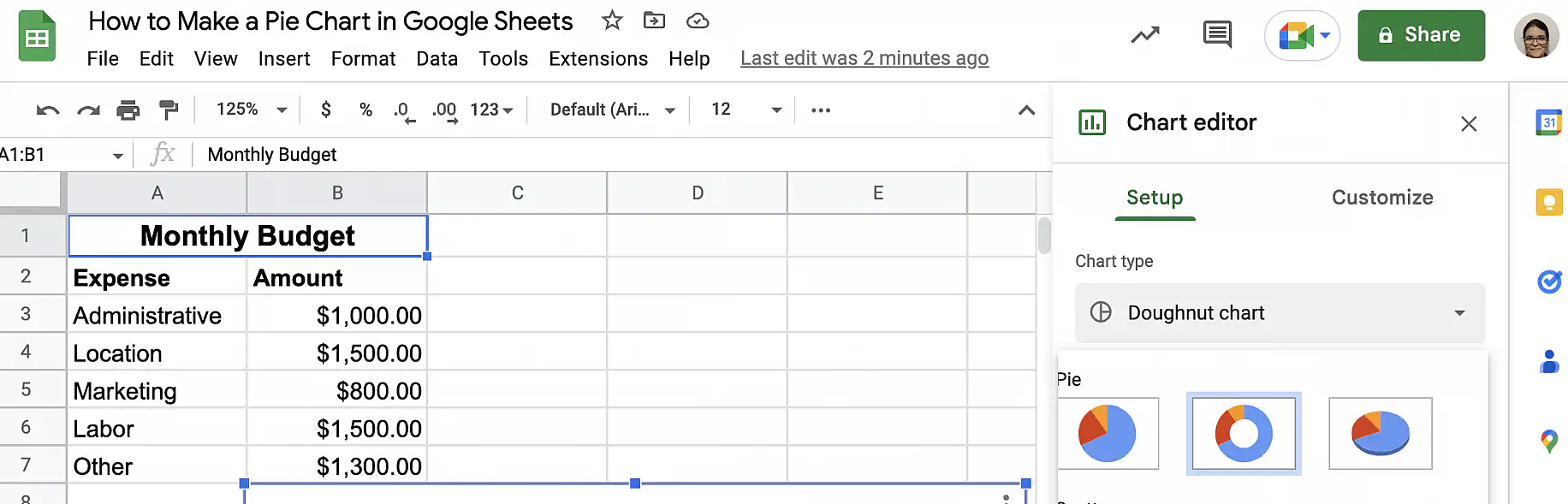
Doughnut chart in Google Sheets — doughnut chart selected in the Pie area

3. That’s it. Your doughnut chart is ready.
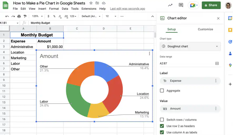
Doughnut chart in Google Sheets — budget data shown as a doughnut chart

Show percentages on the slices

As you saw in the first section, Google Sheets automatically adds labels with the category name and the corresponding percentage. However, you may prefer to display the percentages directly in the corresponding slices of the pie chart.

1. Double-click your pie chart to access the ‘Chart editor’ sidebar.
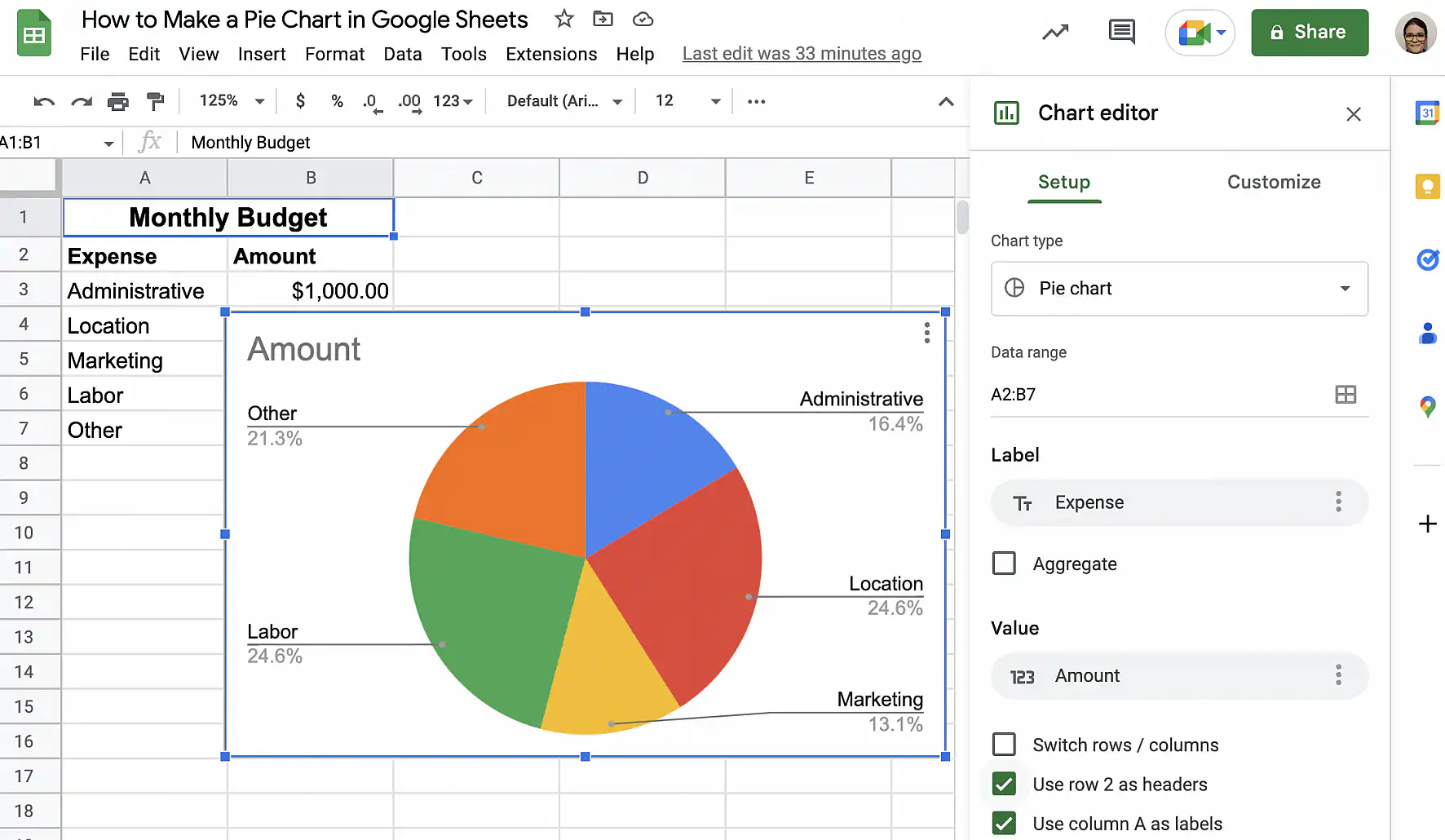
Google Sheets pie chart with percentages — Chart editor open on the Setup tab

2. Click the ‘Customize’ tab, then on ‘Pie chart’ to expand the options.
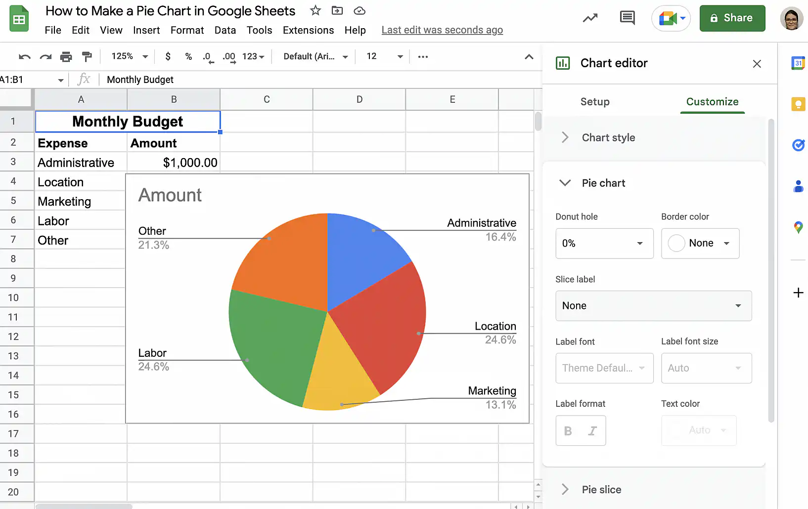
Google Sheets pie chart with percentages — Pie chart options in the Customize tab

3. Click the dropdown menu under ‘Slice label’ and select ‘Percentage’.
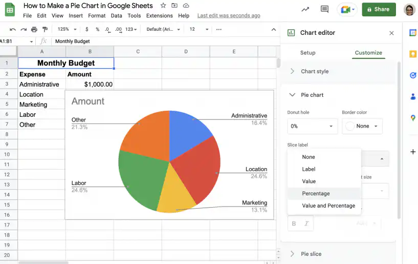
Google Sheets pie chart with percentages — Percentage in the Slice label drop-down menu

4. That’s it. Since the percentages are shown within the pie slices, you don’t need to display them in the legend.
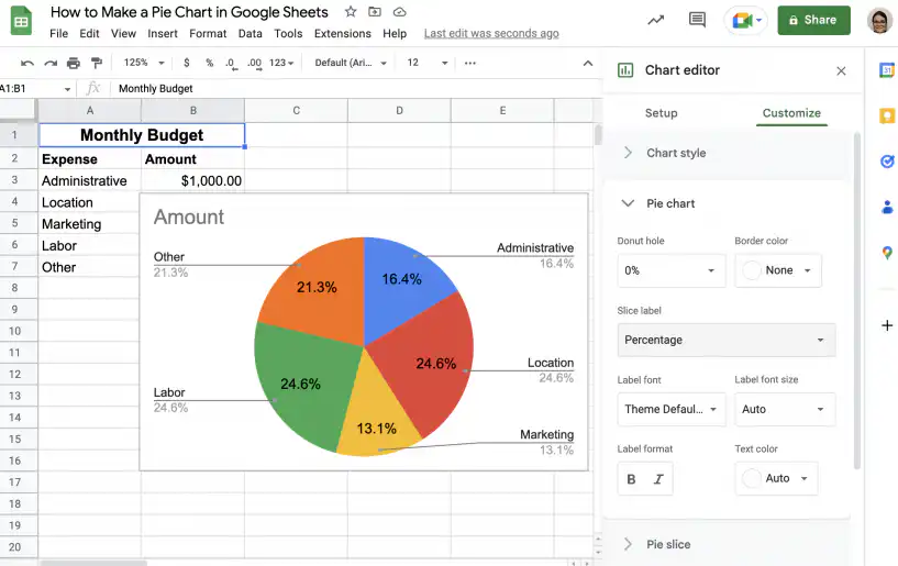
Google Sheets pie chart with percentages — percentages shown inside each slice

5. Under ‘Customize’, click ‘Legend’ to display the options.
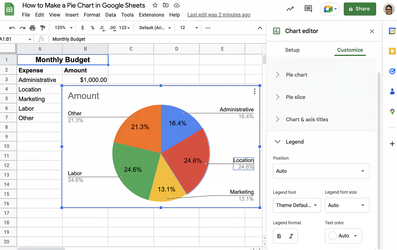
Google Sheets pie chart with percentages — Legend options in the Customize tab

6. Next, click the dropdown menu under ‘Position’ and select one of the options. For this example, I want to display the legend to the left of the pie chart.
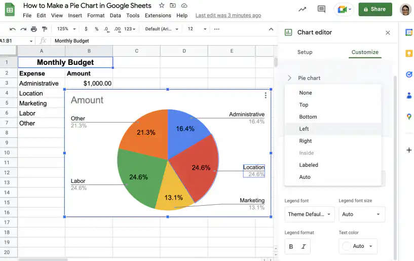
Google Sheets pie chart with percentages — Left chosen in the legend Position menu

7. That’s it. Your pie chart has a legend to identify the different categories, and the percentages are displayed directly in the slices.
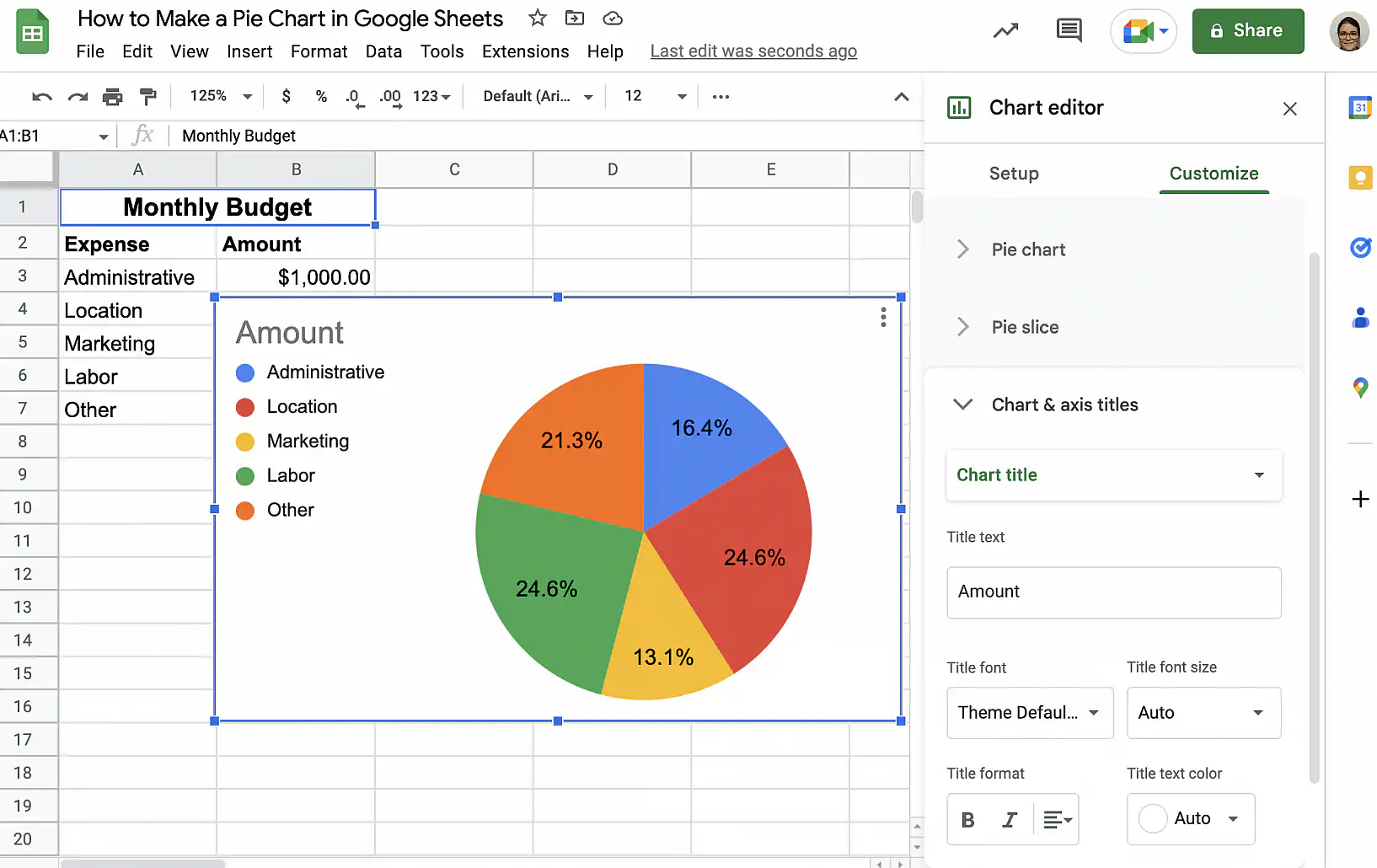
Google Sheets pie chart with percentages — legend on the left and percentages in the slices

Show labels on the slices

You can do this if you prefer not to show the values or percentages and only want the labels.

1. In the ‘Customize’ tab of the ‘Chart editor’, click ‘Pie chart’ to expand the options.
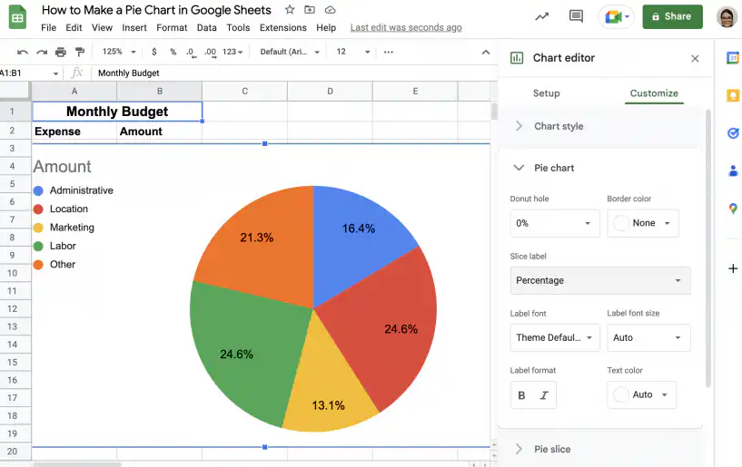
Google Sheets pie chart with labels — Pie chart options expanded in the Customize tab

2. Click the dropdown menu under ‘Slice label’ and select ‘Label’.
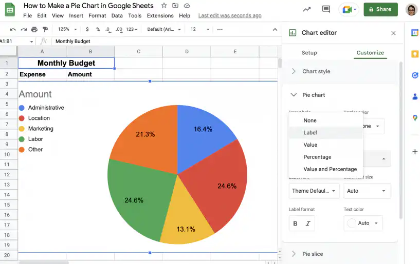
Google Sheets pie chart with labels — Label in the Slice label drop-down menu

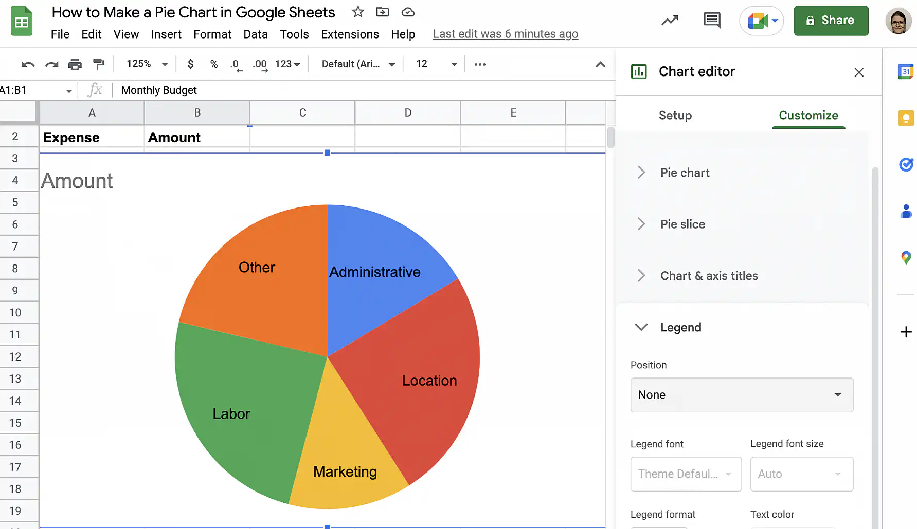
3. That’s it. The labels are now included within each slice. To remove the legend on the left, click ‘Legend’ in the sidebar to expand the options.
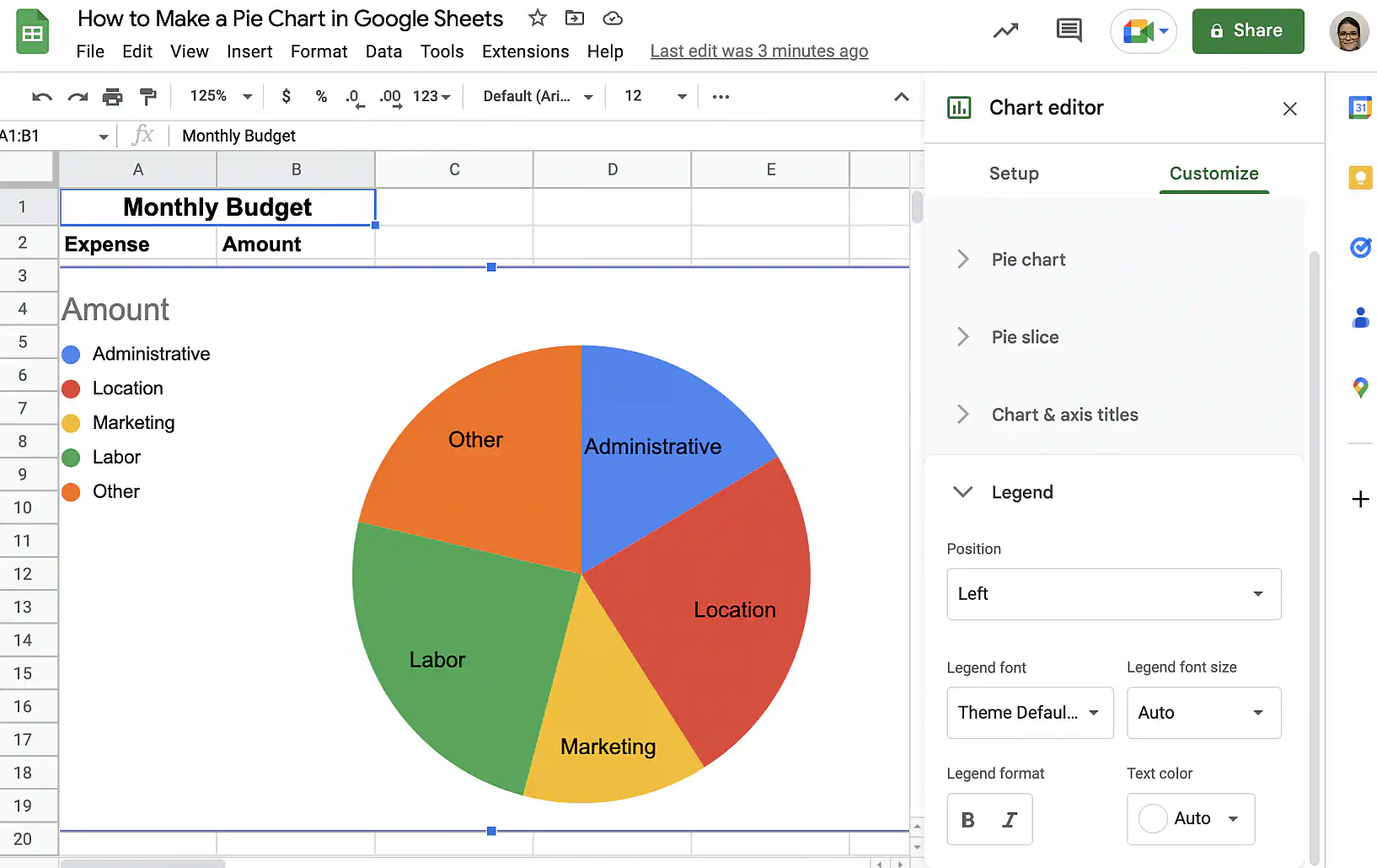
Google Sheets pie chart with labels — category names inside each slice

4. Click the dropdown under ‘Position’ and select ‘None’.
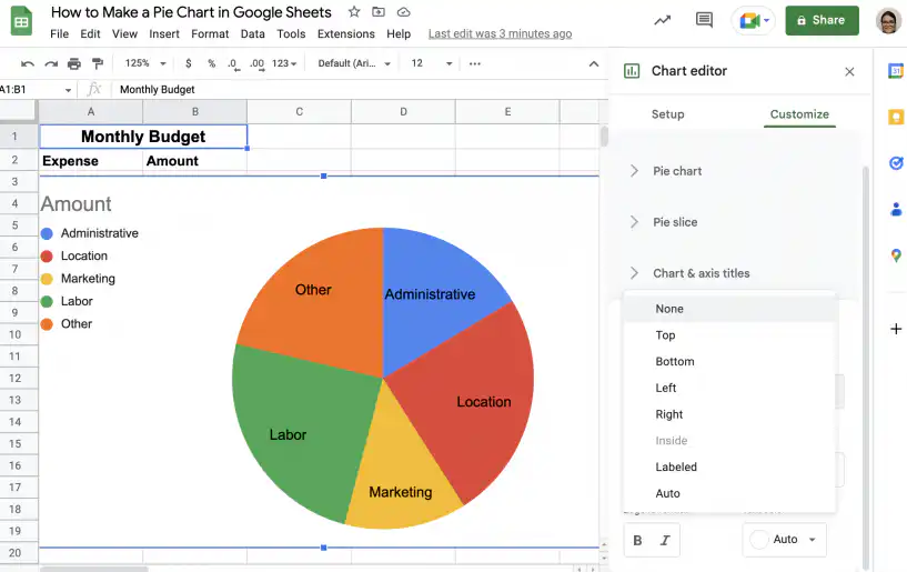
Google Sheets pie chart with labels — None in the legend Position menu

5. That’s it. The legend is gone.

Google Sheets pie chart with labels — chart with the legend removed

Change slice colors and pull out a slice

The screenshots in this section use a different example, a chart of customers by age group, but the steps are the same.

  1. Double-click the chart, open the Customize tab in the Chart editor, and click Pie slice.
  2. Pick a slice from the drop-down menu, then choose a new color under Color.
Google Sheets pie chart — Pie slice options with a color picked for the 18-24 slice
  1. To pull that slice away from the rest of the pie, choose a percentage under Distance from center.
Google Sheets pie chart — one slice pulled out with Distance from center set to 25%

Add a chart title

In the Customize tab, open Chart & axis titles and choose Chart title from the drop-down menu. Type the title under Title text, then set its font, size, format, and color.

Google Sheets pie chart — chart title settings with the title Customers by age group

How to edit a pie chart in Google Sheets

Once you have created a pie chart, editing it is easy. Follow the instructions below to change the chart style or the data range.

Change the chart style

To change the chart’s colors, font, or size:

1. Click the vertical ellipsis in the top-right corner of the chart and choose ‘Edit chart’.
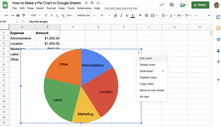
Edit a pie chart in Google Sheets — Edit chart in the chart's three-dot menu

2. In the ‘Customize’ tab, under ‘Chart style’, you can choose the background and border colors, as well as the font.
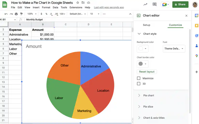
Edit a pie chart in Google Sheets — background color, font and border color under Chart style

3. In addition to changing it to a 3D pie chart, you can check ‘Maximize’ to maximize the amount of space used by the pie chart.
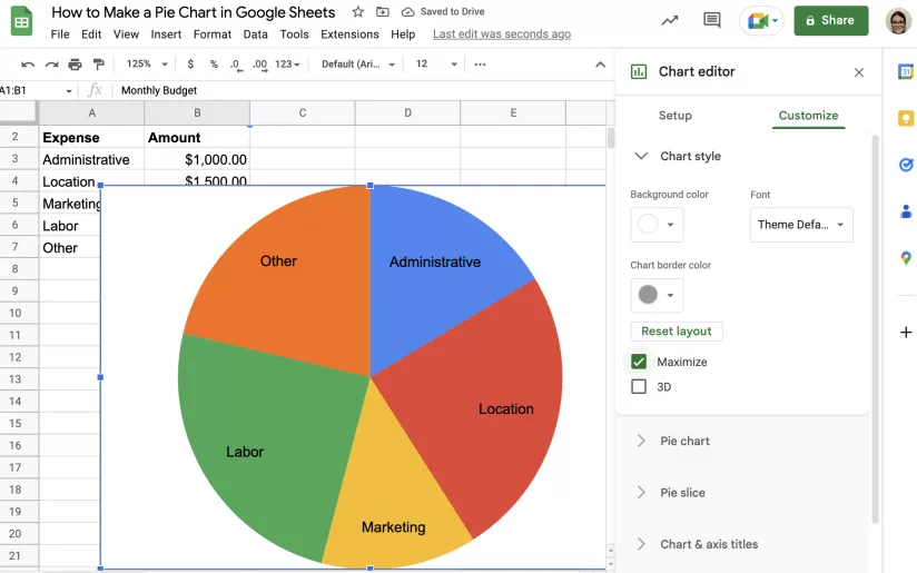
Edit a pie chart in Google Sheets — Maximize ticked under Chart style

Change the data range

To change which cells the chart uses:

1. Right-click anywhere in the chart area and select ‘Data range’ from the menu.
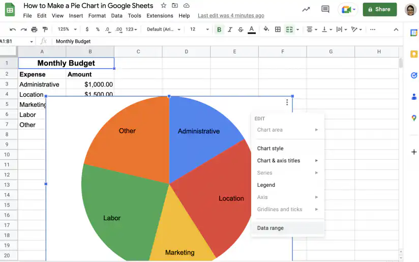
Edit a pie chart in Google Sheets — Data range in the chart's right-click menu

2. You can modify the range manually or use the button shown below to select the range.
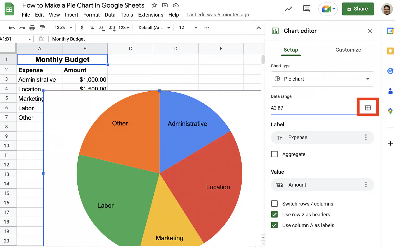
Edit a pie chart in Google Sheets — select data range button next to the Data range field

How to add a pie chart to Google Docs

Google Docs doesn’t build charts on its own. A chart in a document comes from a Google Sheets file, and you can add one in two ways.

  1. To reuse a chart you already made, open your document and go to Insert > Chart > From Sheets. Choose the spreadsheet, select the pie chart, keep Link to spreadsheet checked, and click Import.
  2. To start from scratch, go to Insert > Chart > Pie. Docs adds a sample chart and creates a new spreadsheet for its data. Click the chart, then the link icon, and choose Open source to replace the sample data with yours.

When the data in the spreadsheet changes, click Update on the chart in your document to refresh it.

Conclusion

As you have seen, pie charts visually represent the proportions that make up a whole. This makes them ideal to use when dealing with a small number of categories or values. However, if you have too many categories, it can become visually confusing. In other words, the pie will be divided into so many slices it will be difficult to read and interpret.

You now know how to create a simple pie chart in Google Sheets. Additionally, you know how to make a 3D pie chart, a doughnut chart, how to display percentages, and how to add labels. You also know how to edit your pie chart to change the style or the data range. To learn more about creating charts and tables in Google Sheets, check out our guides on:

For other chart types, see how to make a line graph, create a bar chart, or make a scatter plot in Google Sheets.

To show how numeric values are spread across ranges instead, make a histogram in Google Sheets.

You may also like…

google sheets features and formulas

Top 5 dynamic array formulas in Google Sheets 

Google Sheets has evolved beyond basic spreadsheets. With the introduction of dynamic array formulas, users can now manipulate and analyze...
google sheets features and formulas

Mastering the FILTER Formula: 4 Use Cases with Examples

The FILTER formula in Google Sheets is a versatile tool for extracting data that meets specific conditions. Unlike the QUERY formula,...
google sheets features and formulas

Unlocking the Power of SUMIF and SUMIFS in Google Sheets: 4 real-life use cases

The SUMIF and SUMIFS formulas in Google Sheets are indispensable tools for performing conditional summations. They simplify complex...