Formula parse error in Google Sheets: causes and fixes

If you use spreadsheet formulas frequently, you are no stranger to formula parse errors. These errors occur when a formula is not written correctly. This is a very common problem that affects both beginners and seasoned users.

In this article, we’ll dive deeper into formula parse errors, listing the most common errors and finding ways to fix them.

What is a formula parse error in Google Sheets?

A formula parse error means that Google Sheets cannot read or carry out the instructions in your formula. The errors themselves can be very different, ranging from simple typos, like a missing comma, to mathematical impossibilities, such as trying to divide by zero.

Whenever you encounter a formula error, Google Sheets will display a message. These errors arise when Google Sheets can’t understand your formula. Some of these errors occur when there are syntax mistakes, invalid references or missing arguments.

In order to solve these issues, you need to review and rewrite the formula using the correct syntax and making sure all the references are valid. By understanding common formula errors, you’ll be able to find ways to fix them and ensure data accuracy.

How to fix formula parse errors

Although there isn’t a one-size-fits-all formula to fix these errors, there are some best practices that can help you solve these problems or even prevent them from happening.

Double-check the formula syntax: double-check the formula for any spelling errors, especially in long formulas.

Check all cell references: when you write formulas, you usually reference other cells, ranges and even other worksheets. Make sure all the references are valid and accurate.

Be careful with punctuation marks: when writing a formula, you’ll often need to include parentheses, brackets, commas and quotation marks. It goes without saying that it’s easy to overlook some of these punctuation marks, which can lead to formula parse errors.

Use the right argument separator: Google Sheets separates function arguments with commas or semicolons, depending on the spreadsheet’s locale. In locales that write decimals with a comma, such as Spain, Brazil, or France, =IF(A1>10,"Yes","No") has to be written as =IF(A1>10;"Yes";"No"). A formula pasted with the wrong separator returns a formula parse error. You can check the locale under File > Settings.

Enable formula corrections: Google Sheets has a useful feature for users who need to create formulas frequently. By activating the autocomplete feature, you can enable formula suggestions and corrections. When you activate these features, Google Sheets will automatically autocomplete some formulas, give suggestions or make corrections. Activating these functions is simple. Click Tools, select Autocomplete, and enable these features.

Rule out an outage: if a sheet that worked yesterday suddenly shows errors in formulas nobody changed, check the Google Workspace Status Dashboard before you start debugging.

Formula parse error — Tools menu open on Autocomplete with formula suggestions and corrections enabled

Common formula parse errors

Let’s outline some of the most common formula parse errors now.

#N/A Error

When Google Sheets returns this error, it means that a value is not available. This is a common error message that occurs when Google Sheets can’t return a value that you were looking for.

For instance, when you use functions such as VLOOKUP, QUERY, or MATCH, you will see this message if the value you’re looking for is not available in the specified range.

Below, Google Sheets returned the “#N/A Error” because the value I was trying to find wasn’t available within the specified range of cells.

Formula parse error #N/A — VLOOKUP did not find the name Emma Stone in the list

You can fix this by replacing the value that is not available or checking if you haven’t misspelled the value. You can also wrap the formula in the IFERROR function to return a more informative message if the value you want isn’t available.

#REF! Error

This error occurs when you reference an invalid cell. For this reason, this issue frequently arises when you delete cells or ranges that you are referencing in your formula. You will also see this error message if your formula contains a circular reference. Sometimes, it can happen when you copy and paste a formula with relative references.

It’s a common error when there is a missing reference or the value you’re looking for is outside the ranges you’ve specified.

In this example, my VLOOKUP formula is referencing a cell that is outside the specified range.

Formula parse error #REF! — VLOOKUP asks for column 3 of a two-column range

In order to fix this error, I need to replace all invalid references with valid ones.

#VALUE! Error

This error occurs when your formula has the wrong type of value. In this example, Google Sheets returned an error message because the formula expected number values instead of letters.

Formula parse error #VALUE! — =A2/A3 divides 20 by the text y

When Google Sheets returns this formula parse error, click the cell to see the whole message. It usually says which parameter is causing the error and what data type it should be. Then replace the wrong values.

#NAME? Error

This error indicates that you have referenced an invalid name somewhere in your formula. Whenever Google Sheets doesn’t recognize the name of a built-in function or a named range, it will return this error.

In this example, I’ve misspelled the name of the function. As a result, Google Sheets returned a “#NAME? Error” message.

Formula parse error #NAME? — unknown function AVERAG, a misspelled AVERAGE

Whenever you see this error message, check your formula carefully and correct any misspelled words.

#NUM! Error

This error indicates that your formula contains an invalid number. In general, it occurs when the number is too large for Google Sheets or when it is invalid. In this example, Google Sheets displayed this error message because negative numbers don’t have square roots.

In order to fix this formula parse error, check all the numeric values in your formula to make sure they’re valid. This error also happens when you use LARGE or SMALL and request a number of results larger than the number of existing items.

#ERROR!

Google Sheets will return this error whenever it can’t read your formula at all. When this error occurs, you will only get a “Formula parse error” message.

This error sometimes occurs when you mistype symbols and punctuation marks. Make sure you double-check your formula.

The extra or missing characters could be spaces, punctuation, operators, or alphanumeric characters. For example, missing or extra quotation marks around text values, like John Doe in the formula above, will cause this error message to appear.

#DIV/0! Error

If you see this error message, it means that somewhere in your formula, you’re asking Google Sheets to divide a value by zero. Since that isn’t possible, the result of your formula cannot be calculated.

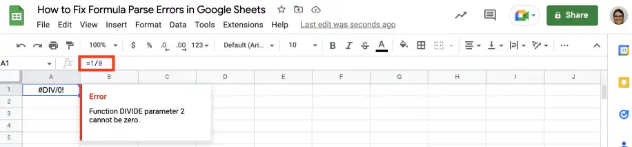
Formula parse error #DIV/0! — =1/0 in A1 with the message that DIVIDE parameter 2 cannot be zero

How to Fix Formula Parse Errors in Google Sheets – #DIV/0! Error

To fix this problem, wrap your formula in the IFERROR function to return a specific value or message when this occurs.

Use formula suggestions and corrections

Don’t forget to use the formula suggestions in Google Sheets whenever you’re not sure about the correct formula syntax. As you can see, you will have access to more detailed instructions and suggestions when you click on the desired function. Google Sheets will even include examples that can help you figure out the correct formula.

Formula parse error help — IF help box with its syntax, an example, and argument notes

Check the built-in function help

In the previous section, you saw an example of a function that could lead to #NUM! errors: LARGE.

1. Double-click to edit your formula and click inside the named function to see suggestions on syntax.

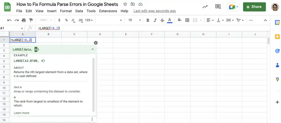
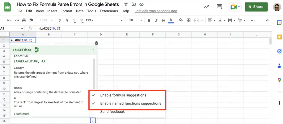
Formula parse error help — LARGE help box with its syntax, an example, and About notes

2. Click on the vertical ellipsis in the bottom-right corner to check that suggestions are enabled.

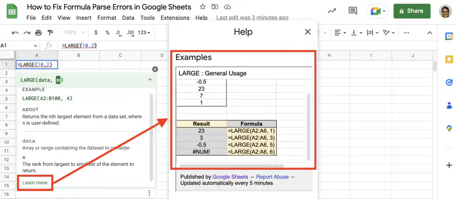
Formula parse error help — help box menu with formula suggestions and named functions suggestions checked

3. Click on ‘Learn more’ for additional help, including examples of general usage.

Formula parse error help — Learn more opening the LARGE help page with example results

How to use the IFERROR function

The IFERROR function returns the expected result if no error is encountered. However, the second argument is returned if an error is encountered, and it can be any value, message, or calculation that you specify. The function will return a blank if the second argument isn’t present. This function is especially useful in cases where errors are predictable, such as using lookup functions or dividing by different values, some of which could be zero.

IFERROR with lookup functions

Follow the steps below to avoid #N/A errors when performing lookups and customize the message that is displayed.

1. In the cell where you want the result of the lookup function, type the IFERROR function.

For the full syntax and more examples, see our guide to the IFERROR formula in Google Sheets. If you only want to replace #N/A and still see every other error, use IFNA instead.

IFERROR formula parse error fix — =IFERROR( typed in A1 with its syntax hint

2. For the first parameter, add your lookup function (in this example, VLOOKUP) with the parameters you want to use. After the closing parenthesis, add a comma.

IFERROR formula parse error fix — VLOOKUP entered as the first IFERROR argument, followed by a comma

3. For the second IFERROR parameter, type in the message (enclosed in quotation marks) that you want to display when the value isn’t found. Alternatively, you can specify a value or a different calculation.

IFERROR formula parse error fix — Missing Value typed as the value_if_error argument

4. Close the parenthesis and press ‘Enter’ to see the result.

IFERROR formula parse error fix — A1 showing Missing Value where the lookup found nothing

How to solve formula parse errors in Google Sheets

That’s how you can fix formula parse errors in Google Sheets. If you want to learn more about other formulas and functions in Google Sheets, we have a wide range of articles to help you. You can start by learning how to use IMPORTRANGE to transfer data from one spreadsheet to another in Google Sheets.

Formula parse error in Google Sheets: what it means and how to fix it