Google Sheets amortization schedule (easy guide)

Google Sheets is known by spreadsheet users as the free online solution to store, structure, and analyze data. It’s also becoming more widely used among finance experts, as it has powerful built-in financial functions that allow you to perform from simple to more complex calculations, whether it’s for your business or personal use.

For example, you can use Google Sheets PMT, PPMT, and IPMT functions to calculate how much you’ll pay to settle a loan or investment, including the principal and interest. Moreover, you can build your loan amortization schedule to check how monthly payments impact the final amount.

In this article, you’ll learn what the Google Sheets loan amortization schedule is and how to create a standard one and a loan amortization schedule, including extra payments.

What is a Google Sheets loan amortization schedule?

Loan amortization is a process aimed at paying off the interest payment for a given period, and then the remaining amount is put towards reducing the principal payment. As these payments are periodic, you can schedule them beforehand to see the principal and interest amount you’ll need to pay until you fully settle the loan.

In Google Sheets, you can use the PMT, PPMT, and IPMT functions to create your own loan amortization schedule.

PMT, PPMT, and IPMT functions

Before diving into the steps to create your loan amortization schedule, let’s see how these functions are expressed as a formula and what each argument means.

PMT syntax

=PMT(rate, number_of_periods, present_value, future_value, end_or_beginning)

rate is the interest rate for the payment period.
number_of_periods is the number of payments you need to make to settle the loan.
present_value is the principal amount.
future_value is an optional argument that represents the future value that will remain after making the final payment.
end_or_beginning is an optional argument that specifies if the payments are due at the end (represented by “0”) or start (“1”) of each period. This value is set to “0” by default.

PPMT syntax

The PPMT syntax is almost the same as the PMT, but it includes the period argument:

=PPMT(rate, period, number_of_periods, present_value, future_value, end_or_beginning)

period refers to the amortization period. For example, if you have 60 periods, this argument should be represented by any number between 1 – 60.

IPMT syntax

Although the syntax is the same, whereas the PPMT is used to calculate the principal amount, the IPMT function calculates the interest amount, so you can determine the proportions for each payment.

=IPMT(rate, period, number_of_periods, present_value, future_value, end_or_beginning)

How to create a loan amortization schedule in Google Sheets?

Now that you know the syntax for each function used to create your loan amortization schedule, let’s begin by preparing the amortization table format.

How to prepare the loan amortization schedule table format?

Before using the functions, make sure you set up the data and the table format for the amortization schedule. This is how you can prepare the loan amortization schedule.

1. Enter the values for your amortization schedule, including the rate, number_of_periods, and the present_value.

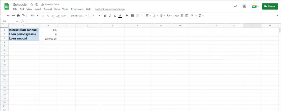
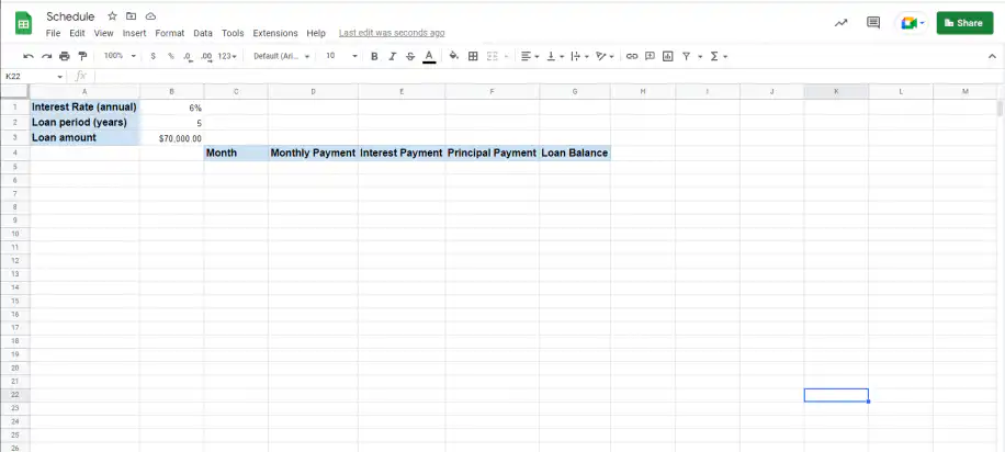
Google Sheets amortization schedule — annual interest rate 6%, loan period 5 years and loan amount $70,000.00 in a sheet named Schedule

2. Create a table with 5 columns, each corresponding to the data required to create the schedule.

Google Sheets amortization schedule — Month, Monthly Payment, Interest Payment, Principal Payment and Loan Balance column headers

How to fill the loan amortization schedule using the PMT, PPMT, and IPMT functions?

As you saw in the previous section, you’ll need to adapt three formulas to your data. This is how to fill the loan amortization schedule using the PMT, PPMT, and IPMT functions.

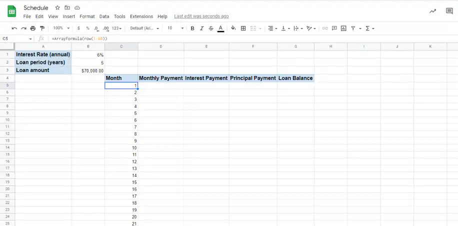
1. Depending on the number_of_periods, you can use this formula to quickly fill in the first column, =ArrayFormula(row(cell range)), as shown below.

Google Sheets amortization schedule — ArrayFormula with ROW numbering the Month column from 1

2. To fill in the data for “Monthly Payment”, use the PMT formula, including only the first 3 arguments. Once you do, press “Enter”.

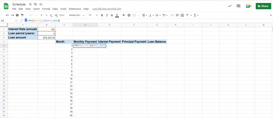
Google Sheets amortization schedule — PMT formula typed in the first Monthly Payment cell

NOTE: Make sure to divide the rate by 12 and multiply the loan period (if in years) by 12, as there are 12 months in a year.

3. To fill in the data for the whole column, add the array formula to the PMT formula. Press “Enter” to apply the formula.

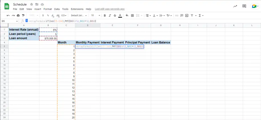
Google Sheets amortization schedule — ArrayFormula wrapped around PMT in the first Monthly Payment cell

4. Your schedule should now show the Monthly Payment for each month.

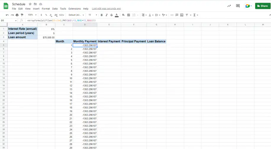
Google Sheets amortization schedule — Monthly Payment column filled with the same payment for every month

5. To calculate the “Interest Payment”, type in the array formula and the IPMT formula, as shown below.

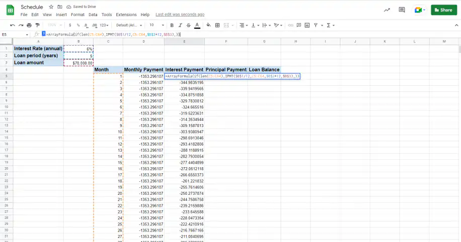
Google Sheets amortization schedule — ArrayFormula with IPMT filling the Interest Payment column

6. To calculate the “Principal Payment”, type in the array formula and the PPMT formula, as shown below.

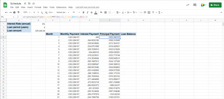
Google Sheets amortization schedule — ArrayFormula with PPMT filling the Principal Payment column

7. To calculate the “Loan Balance” you need to subtract the first “Principal Payment” from the initial loan amount. If the values are negative, add a “+” not “minus” to subtract. Press “Enter” to obtain the result.

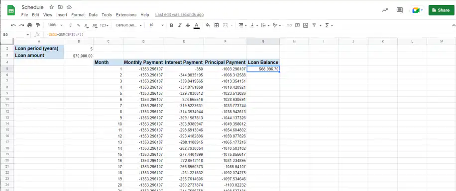
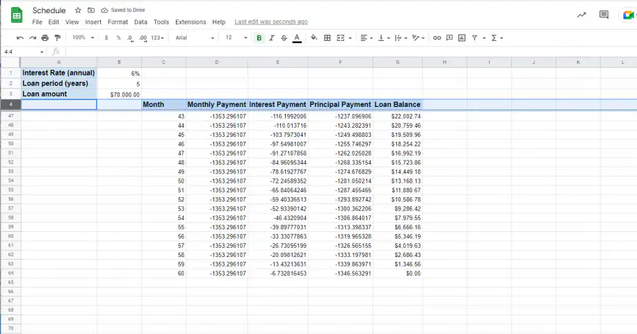
Google Sheets amortization schedule — first Loan Balance cell after subtracting the first principal payment

8. Grab the cell where you included the loan balance formula, and drag it down until the last period. If you did it correctly, the last cell should contain the value of “0”, as shown below.

Google Sheets amortization schedule — Loan Balance column dragged down to $0.00 at month 60

How to create a loan amortization schedule with extra payments in Google Sheets?

As you’ve seen, creating a loan amortization schedule in Google Sheets using PMT, PPMT, and IPMT functions is a straightforward process. However, if you need to include extra principal payments, you’ll need to follow different steps.

1. Include another row with “Payment”, under the three main input values and a new column for “Extra Payment”. You’ll need to leave an empty cell under each column name, except for the “Loan Balance”.

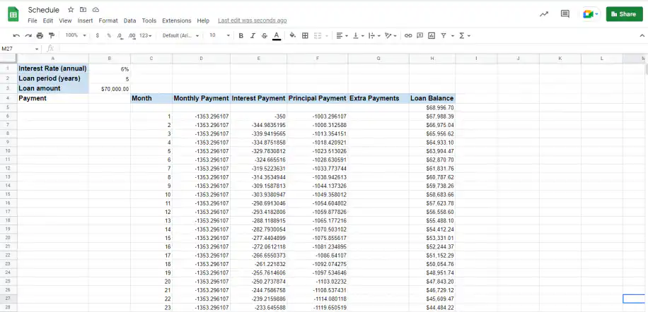
Google Sheets amortization schedule with extra payments — new Payment row and Extra Payments column added to the table

2. This time, you’ll calculate the periodic payment in the cell that corresponds to “Payment”. You can use the PMT formula, using the first three arguments, as shown below.

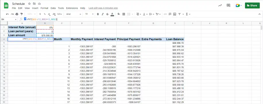
Google Sheets amortization schedule with extra payments — PMT formula in the Payment cell under the loan amount

3. Include the value of the loan amount in the first cell of the “Loan Balance” column, by typing the "=" sign followed by the cell reference. Press "Enter".

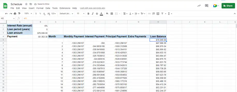
Google Sheets amortization schedule with extra payments — first Loan Balance cell showing the $70,000.00 loan amount

4. To obtain the PMT value from the new “Payment” value, you’ll need to combine the IF formula with the PMT formula, as shown below. Once you type it in, press “Enter” to apply.

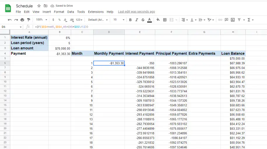
Google Sheets amortization schedule with extra payments — IF and PMT formula returning $1,353.30 in the first Monthly Payment cell

NOTE: This combination of IF+PMT checks the balance column in the row above. For example, cell D6 will check the value in cell H5. If the value in the “Payment” is less than the “Loan Balance” value, the PMT value remains the same. If the PMT is more than the balance value, the IF formula will run the second part of the formula.

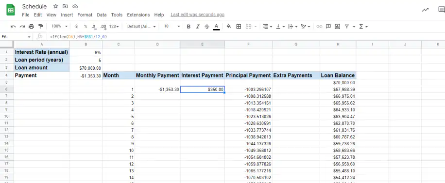
5. To obtain the interest payment, combine the IF formula with the IPMT, as shown below.

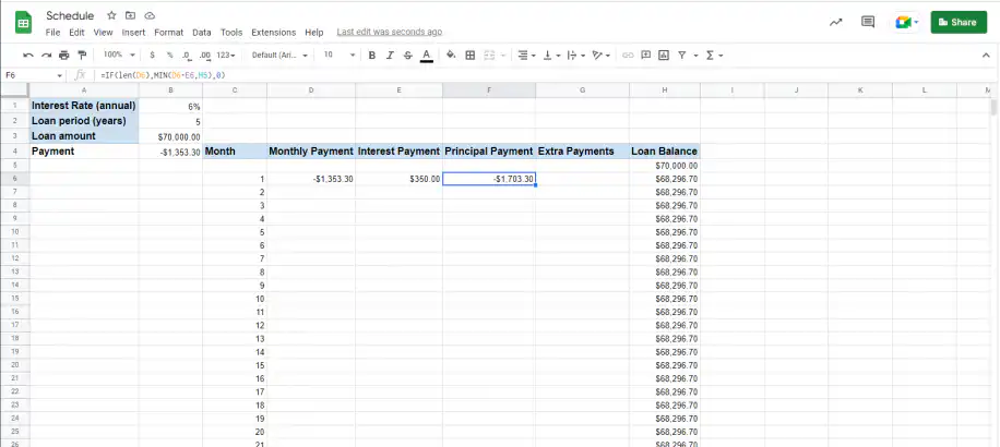
Google Sheets amortization schedule with extra payments — IF and IPMT formula returning $350.00 in the first Interest Payment cell

6. To obtain the principal payment, you’ll also need to combine the IF formula with the PPMT, as shown below.

Google Sheets amortization schedule with extra payments — IF and PPMT formula in the first Principal Payment cell

7. Include the amount in “Extra Payments” and drag it down to copy that same amount.

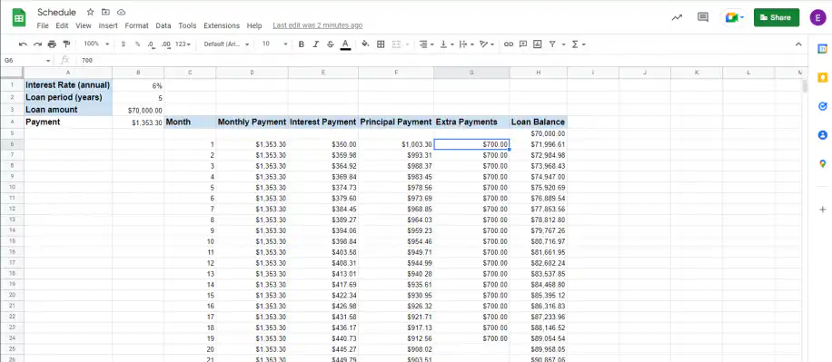
Google Sheets amortization schedule with extra payments — $700.00 copied down the Extra Payments column

8. Use this formula to balance the loan, in the corresponding cell, right under the initial loan amount, as shown below.

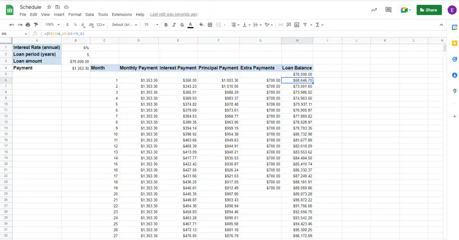
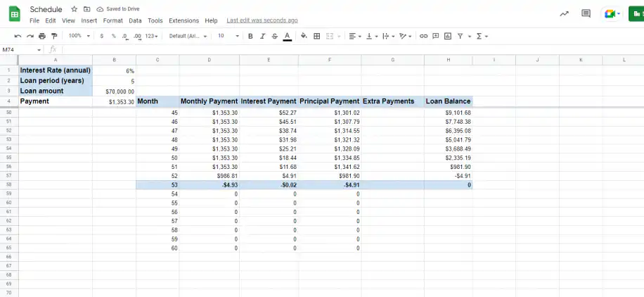
Google Sheets amortization schedule with extra payments — loan balance formula in the cell under the $70,000.00 starting balance

9. Drag down until you reach “0”. As you can see, the rest of the cells have changed, and you now know how many payments you’ll need to make, with the extra payments, to pay off the loan.

Google Sheets amortization schedule with extra payments — Loan Balance reaching 0 at month 53 with zeros in the months after

Conclusion

As you’ve seen, the amortization schedule in Google Sheets can be customized according to the type of loan by simply changing the values. Having a loan amortization schedule can also help you determine the interest and principal payments on your loan over a specified period. This way, you’ll be able to see how payments related to the interest decrease, whereas those related to the principal amount increase.

You should now have a better understanding of what the Google Sheets loan amortization schedule is, as well as how to prepare a loan amortization schedule using the PMT, PPMT, and IPMT functions. In case you need to include extra payments, you’re also ready to adapt the amortization schedule to any extra payments.

If you are paying off more than one loan, these debt reduction spreadsheets help you decide which balance to clear first.