Linear regression in Google Sheets (+ examples)

Google Sheets provides functions for many data analysis methods, including linear regression. This method is frequently used to quantify the relationship between a dependent and an independent variable. In other words, if you’ve noticed a linear trend in your data, you can forecast future values using the linear regression method. The LINEST function in Google Sheets allows you to perform both simple and multiple linear regression on the known values for your variables. You can quickly find the slope and the intercept, as well as other regression statistics.

In this article, you will learn about the LINEST function and syntax, as well as how to use it for regression analysis in Google Sheets. You will see examples of how to use it when you have one explanatory variable – simple regression – and how to use it when you have multiple explanatory variables – multiple regression.

LINEST function syntax

The LINEST function has four parameters, and only the first is required.

=LINEST(known_data_y, [known_data_x], [calculate_b], [verbose])

• known_data_y* (Required): The known values for the response or dependent variable (y).
• known_data_x (Optional): The known values for the explanatory or independent variable (x).
• calculate_b (Optional): Indicates whether the y-intercept (b) should be calculated. The default value is “TRUE”, which is what we want for linear regression.
• verbose (Optional): Indicates whether you would like to see additional regression statistics or just the slope and intercept. The default value is “FALSE”.

This means you can use it to calculate the trend in values for your dependent variable even if you don’t have an independent variable. However, you can also use it when you have multiple independent variables that need to be considered. This makes it a very flexible and useful function.

In the following sections, you will learn how to use the function for both simple and multiple linear regression.

How to use the LINEST function in Google Sheets (simple regression)

Follow the instructions below to run a simple linear regression analysis in Google Sheets. For this example, I will use the sales amount as the response or dependent variable. The explanatory or independent variable is the amount spent on paid advertising.

1. Open the Google Sheets file with the data for the explanatory and response variables.

2. Type "=LINEST(" in an empty cell and you will see the help pop-up. Select the array of cells with the known values for the response variable, "sales_amount".

3. After the comma, select the range of known values for the independent variable, “paid_ads”.

4. I will set the last two parameters to “TRUE”, as I want “b” to be calculated, and I want to see more regression statistics than the slope and intercept. Remember to close the parenthesis and press Enter.

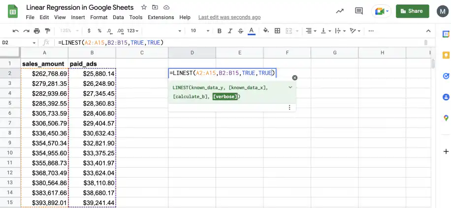
5. That’s it. All the regression statistics are available in your spreadsheet, but which is which? In the next step, I include labels for each of the statistics provided.

6. Below, I have identified the statistics provided by the formula when the “verbose” parameter is “TRUE”. If the parameter is set to “FALSE” or left blank, only the “slope” and “intercept” statistics are provided.

How to run a multiple linear regression in Google Sheets

Follow the instructions below to run multiple linear regression analysis in Google Sheets. I will build on the previous example by adding a second independent variable. The dependent variable is still the sales amount, but the explanatory variables are now the amount spent on paid advertising and the amount spent on sales salaries.

1. Open the Google Sheets file with the data for the response variable and both explanatory variables.

2. In an empty cell, type "=LINEST(" and you will see the help pop-up. Select the array of cells with the known values for the response variable, "sales_amount".

3. After the comma, select the range of known values for the independent variables, “paid_ads” and “sales_salaries”.

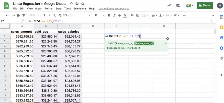
4. The third parameter is set to “TRUE”, as I want “b” to be calculated. I also want to see all the regression statistics, so the last parameter is also “TRUE”. Remember to close the parenthesis and press “Enter”.

5. That’s it. The statistics for the multiple regression are available in your spreadsheet. In the next step, I will identify the statistics with labels.

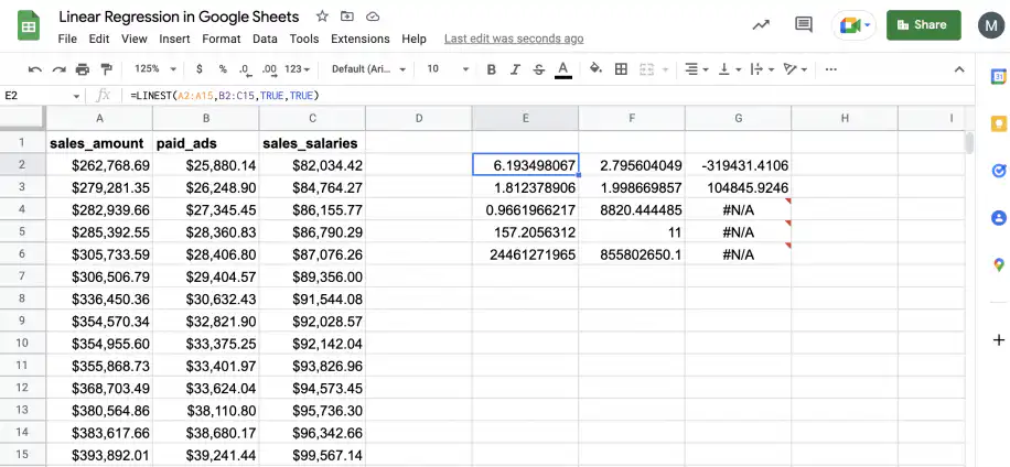
6. Below, “s.error” is the standard error. The cells with “#N/A” can be ignored, as there is no error: the cells are simply not needed.

How to read the LINEST output array

With “verbose” set to “TRUE”, LINEST returns five rows of statistics. Rows 1 and 2 have one column for each independent variable plus one for the intercept. Rows 3 to 5 only use the first two columns.

• Row 1: the slope for each independent variable, then the intercept (b).
• Row 2: the standard error of each slope and of the intercept.
• Row 3: the coefficient of determination (r²) and the standard error of the y estimate.
• Row 4: the F statistic and the degrees of freedom, which you need to test whether the relationship is significant.
• Row 5: the regression sum of squares and the residual sum of squares.

In the simple example, the slope is about 9.37, so each extra dollar spent on paid ads goes with about $9.37 more in sales. The r² of 0.93 means the line explains 93% of the variation in sales.

In a multiple regression, LINEST lists the slopes in reverse order. The first value, 6.19, belongs to sales_salaries, the last x column, and 2.80 belongs to paid_ads. The #N/A cells in rows 3 to 5 are just the columns those rows don’t use.

For a simple regression, r² is also the square of the value the CORREL function returns. To see the fitted line, plot the data in a scatter chart and add a trendline. If you’d rather use a menu than a formula, the XLMiner Analysis ToolPak add-on runs the same regression.

Conclusion

As you have seen, linear regression analysis is easy using the LINEST function in Google Sheets. Whether you have one or multiple independent variables, you can quickly find the slope and the intercept.

However, you could also find those using the SLOPE and INTERCEPT functions. The difference is that LINEST can also provide a lot of additional regression statistics, which will allow you to perform a full analysis. These include standard errors for slope, intercept, and y-estimate, as well as the coefficient of determination, F statistic, degrees of freedom, and the regression and residual sums of squares.

You now know how to find simple and multiple linear regression in Google Sheets using the LINEST function. You also know how to identify the statistics represented by the function’s output, so you can quickly interpret the results. To learn more about performing data analysis in Google Sheets, check out our related article on how to perform what-if analysis in Google Sheets.

To predict a future value from the same kind of data, use the Google Sheets FORECAST function. It fits a straight line to your data and returns the y value for a new x.