How to make a line graph in Google Sheets

A line graph, also called a line chart, shows how one or more values change over time. Each data point is a marker, and a line joins the markers so you can see the trend at a glance. In Google Sheets, you can build one from a table with dates or periods in one column and values in the next.

This guide shows you how to make a line graph in Google Sheets with a single line and with multiple lines, and then how to customize it. You’ll also see the three line chart types in Google Sheets and how to add a vertical line that marks a date on the chart.

What is a line graph in Google Sheets?

Google Sheets offers various types of charts to visualize your data. One of these is the line graph, which is ideal for illustrating changes to one or more variables over time. Usually, the X-axis shows the time units, while the Y-axis shows the units of the other variables.

If you want to visualize a single variable to see how it changes over time, you can use a line graph with a single line. However, you can easily show multiple lines on the same line graph, provided they are in the same units.

How to make a line graph in Google Sheets

Follow these steps to make a line graph with one line or with several lines.

Make a line graph with a single line

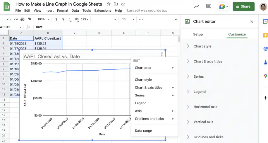
Let’s start by creating a single line graph in Google Sheets, showing changes to Apple’s closing price in January.

1. Open Google Sheets to the file with your data.

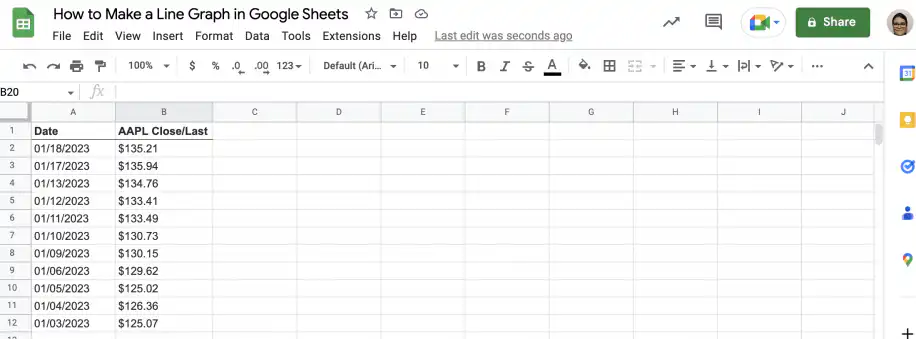
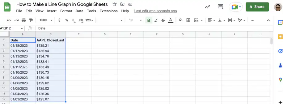
2. Select the data you want to include in the line graph. In this case, it’s the date and stock price data.

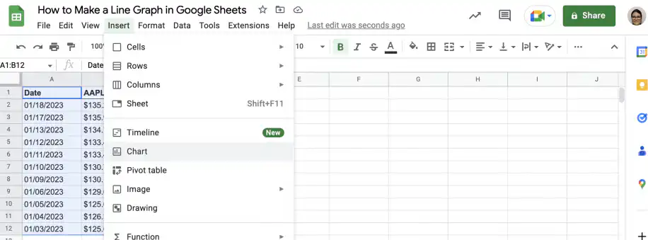
3. Go to Insert > Chart.

4. Google Sheets usually recognizes the type of data and selects the appropriate chart type. However, if it doesn’t, go to the ‘Chart editor’ sidebar and select the ‘Line chart’ under ‘Chart type’.

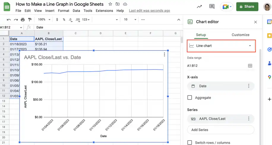
5. You can edit and customize the chart by right-clicking on the chart or from the ‘Customize’ tab in the ‘Chart editor’. The section on how to customize a line graph, further down, covers the main options.

Make a line graph with multiple lines

Now that you know how to make a single-line graph, let’s see how to create one with multiple lines. Let’s add two more lines to the line graph created in the previous section: the closing prices for Microsoft and Cisco.

1. Open the spreadsheet with your data in Google Sheets.

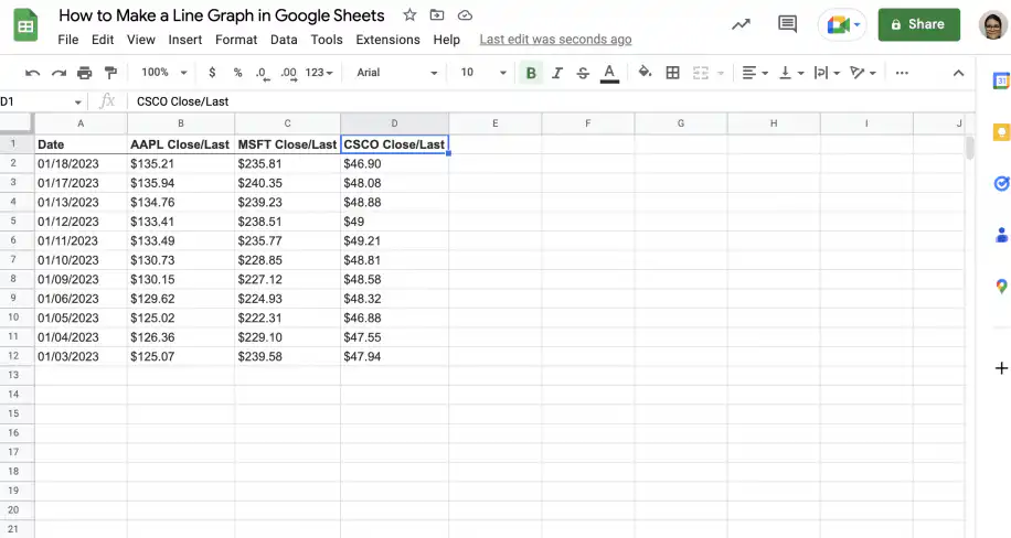
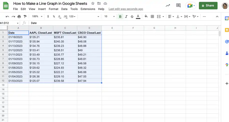
2. Select the data you want to include. In this case, the date and the three stock prices.

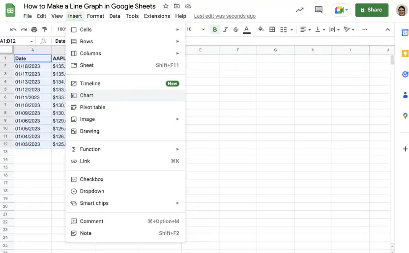
3. Go to Insert > Chart.

4. If Google Sheets doesn’t do it automatically, select ‘Line chart’ under ‘Chart type’ from the sidebar.

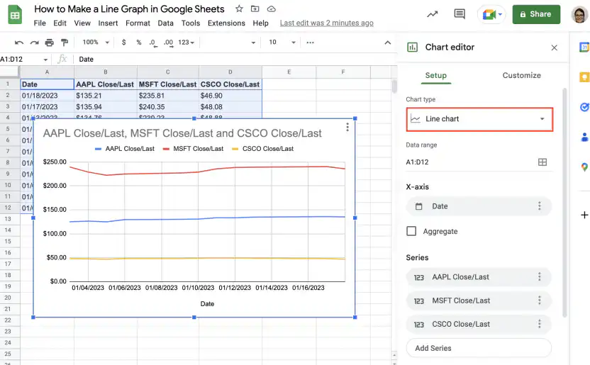
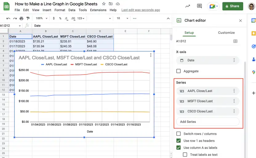
5. As you can see, this graph has three lines: one for each stock price. You can add or remove series or lines from the ‘Setup’ tab in the ‘Chart editor’.

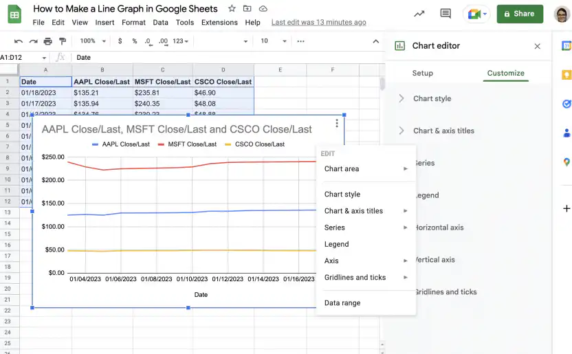
6. To customize or edit the chart, use the ‘Customize’ tab in the ‘Chart editor’ or right-click on the chart to see a menu.

How to customize a line graph in Google Sheets

To change how your line graph looks, double-click it and open the Customize tab in the Chart editor. The screenshots in this section use a different example, yearly revenue for three branches, but the options are the same for any line graph.

1. Open Chart style to change the background color, the font, and the chart border color.

2. Open Chart & axis titles, choose Chart title, and type the title. You can also set its font, size, format, and color.

3. Open Series to change the color, opacity, dash type, and thickness of the lines. To show a marker on each data point, pick a point size and a point shape.

4. Open Legend to move the legend, for example to the bottom of the chart, and to set its font, size, and color.

5. Open Vertical axis and set Min and Max. When the lines sit close together, a tighter range spreads them out. In this example, a range of 4 million to 11 million instead of 0 to 12.5 million makes the differences between the branches easier to see.

6. Open Gridlines and ticks to add or remove gridlines and ticks. Here, the major gridlines of the vertical axis are turned off, which removes the horizontal lines across the chart.

How to make a line chart in Google Sheets

To make a line chart in Google Sheets, pick one of the three options under Line in the Chart type menu: line chart, smooth line chart, or combo chart.

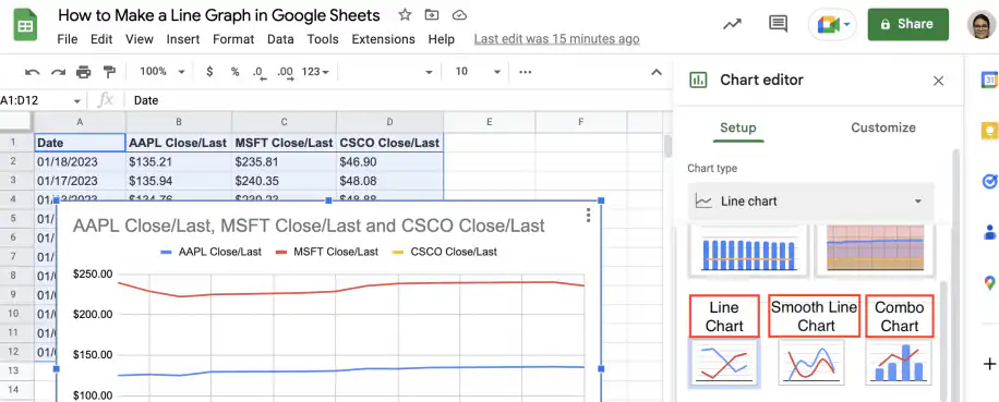
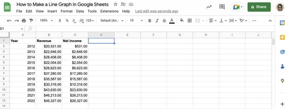
Let’s see how the line chart and the smooth line chart differ by creating each type for the same set of variables, which include year, revenue, and net income. Finally, you will see how to use a combo chart to represent change over time using bars for one variable and a line for the other.

Line chart

Follow the steps below to create a line chart showing changes to revenue and net income over time.

1. Open Google Sheets to the file containing your data.

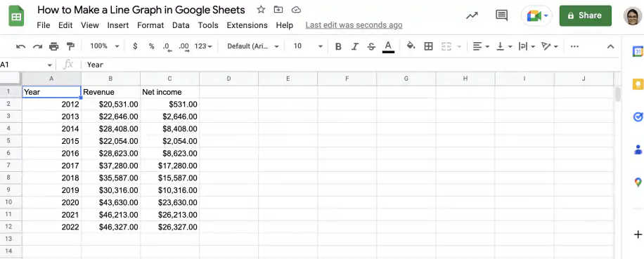
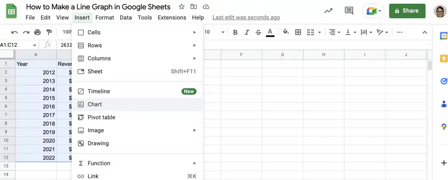
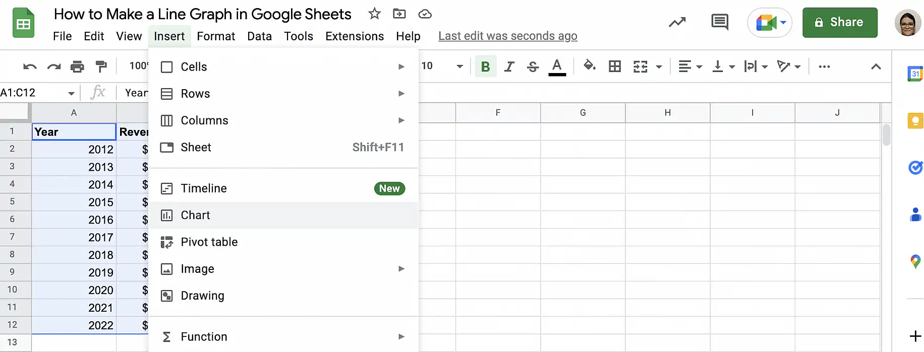
2. Select the data you want to include and go to Insert > Chart.

3. Make sure that the chart type is ‘Line chart’.

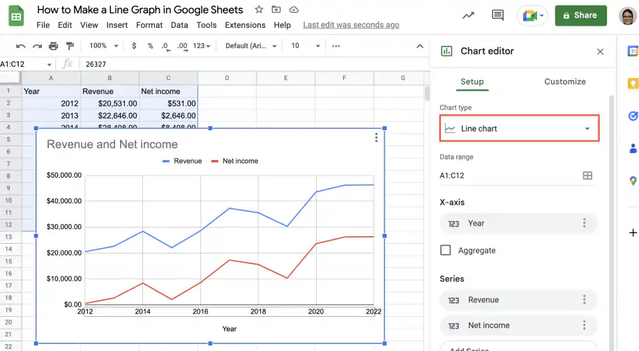
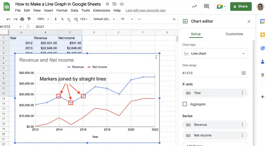
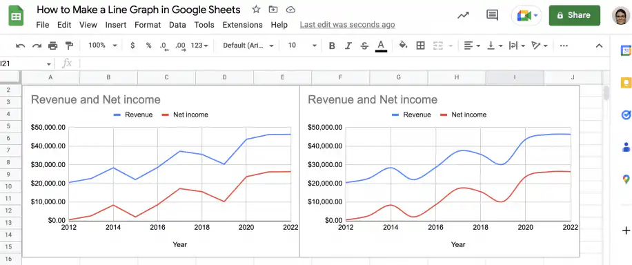
4. As you can see below, each data point is represented by a marker, and these are joined by straight lines.

Smooth line chart

Follow the steps below to create a smooth line chart showing the same data as the previous example: revenue and net income over time.

1. Using the chart from the previous example, go to the ‘Setup’ tab in the ‘Chart editor’.

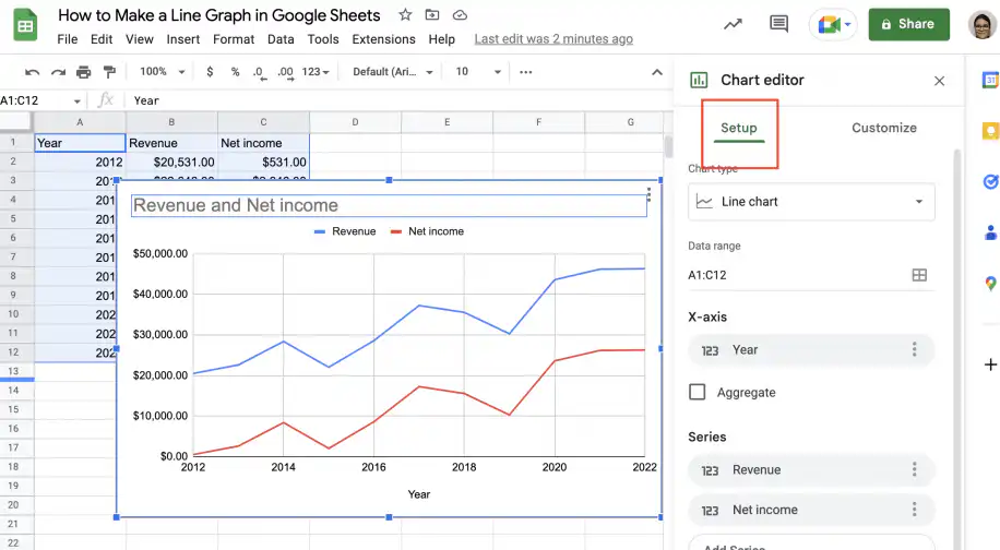
2. Under ‘Chart type’, change the selection to ‘Smooth line chart’.

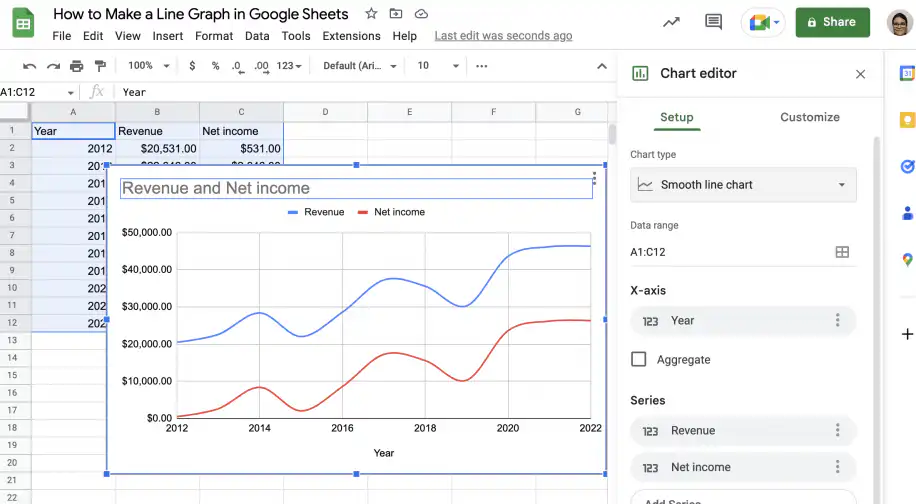
3. As you can see, the lines joining the data markers are now smooth, which means the chart shows a slightly distorted view of reality. You should be especially careful using this type of chart with small datasets, as the distortion will be greater.

Combo chart

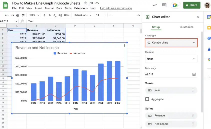
Finally, let’s see how you can use the combo chart to represent each variable using a different method: one variable is represented by bars, while the other is represented by markers joined by a line. Follow the instructions below to make a combo chart showing revenue and net income over time.

1. Open the spreadsheet with your data in Google Sheets.

2. Select the data you want to include and go to Insert > Chart.

3. Select the ‘Combo chart’ from the ‘Chart editor’. Revenue is represented by the blue bars and net income by the red line.

How to add a vertical line to a Google Sheets chart

Google Sheets has no setting that draws a vertical line on a chart, for example to mark a launch date or the start of a quarter. You can get one with a helper column and a combo chart.

1. Add a helper column next to your data.
2. In the row of the date you want to mark, enter a value at least as high as the largest value in the chart. Leave the other cells of the helper column empty.
3. Select the data, including the helper column, and go to Insert > Chart.
4. In the Setup tab of the Chart editor, set Chart type to Combo chart.
5. Open the Customize tab, click Series, and pick the helper series. Set its Type to Columns, and set every other series to Line.
6. Under Vertical axis, set Max to the value you entered in the helper column, so the column reaches the top of the chart.

The helper series now shows as a single thin column at the date you picked, which reads as a vertical line. The column gets thinner as you add rows, so this works best with daily or weekly data. The helper series also appears in the legend, so give its header a clear label, such as Launch.

Conclusion

As you have seen, line graphs are a great way to visualize changes to variables over time. You can create graphs showing one or multiple variables to see the evolution of each and easily compare them. While using a smooth line chart may look a little prettier, you should be careful not to use it with very small datasets, as manipulating the data in this way can lead to a distorted view.

You now know what line graphs are and how to use them in Google Sheets. You have step-by-step instructions on how to create a line graph using a single line or variable, as well as how to make one using multiple lines to represent different variables. You also know how to customize the chart, how the three line chart types in Google Sheets differ (line chart, smooth line chart, and combo chart), and how to mark a date with a vertical line. Finally, you’ve seen examples of line charts showing changes to stock closing prices, as well as revenue and net income over time.

To learn more about tables and charts in Google Sheets, check out these guides:

• How to make a table in Google Sheets
• How to create a pivot table in Google Sheets
• How to make a pie chart in Google Sheets

For other chart types, see how to create a bar chart or make a scatter plot in Google Sheets.

If the numbers behind your line graph come from several spreadsheets, Sheetgo can bring them into one sheet on a schedule. Your chart then updates on its own, and the data stays organized and AI-ready.