How to use the SUMIF function in Excel

People often use Microsoft Excel for highly sophisticated and complex calculations. At other times, you may just want to use Excel to add up certain data points. While the SUM function is perfect for doing just that, what happens when you don’t want to tally all the data in your spreadsheet? In that case, you can use the SUMIF function to tell your spreadsheet which data to add, and which to ignore.

Syntax

• range is the group of cells you wish to add up
• criteria is the characteristic that will decide whether or not each cell gets included. This can be an expression, number, cell reference, or text string
• sum_range is an optional parameter that specifies the cells to add up. If left out, the default is to add up the cells in the range that meet the criteria

How to use the SUMIF Excel function

I’ll show some examples to demonstrate how to use the SUMIF Excel function to add up data in any way you want.

In the examples, I use data from a fictional department store, with sales numbers for different employees in various departments.

Critera with logical operator

Take a look at the first example below. I want to find the total number of sales by all employees who had more than $10,000 in sales.

Right away, you can see that I can’t simply add up the sales numbers in column C. Doing this would include the sales of employees who had less than $10,000 in sales.

I could manually select all the sales numbers that fit my criteria, but this would be time-consuming, especially in a large dataset. So instead, I type =SUMIF(C2:C11,">10000").

I use the greater than “>” logical operator in this example, but you can use any of the logical operators shown below.

Just make sure to put the criteria in quotation marks when using a logical operator.

Critera as text string

In the next example, I’ll show a different type of criteria. This time, I’m filtering the data based on the department in which the employee works.

Specifically, I want to determine the total sales of employees in the Food department. I achieve this with the formula =SUMIF(B2:B11,"Food",C2:C11).

There’s a couple of differences between these two examples. Firstly, the criteria in the second example is not numerical – it’s a text string. The function searches the range for the string “Food” and adds up all the sales of the corresponding cells.

That brings me to the second difference: because I’m adding up data from a different column than where I’m applying the criteria, I have to use the sum_range parameter.

Criteria as cell reference & multiple SUMIFs

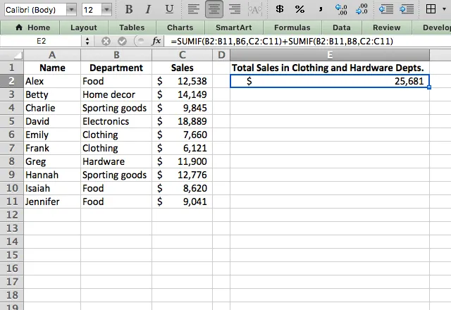
Now I’ll show another way to specify your criteria: using a cell reference. Instead of typing out the department I want, I’ve just selected a cell that contains that department as my criteria parameter. This saves a bit of time compared to typing out the text string.

You’ll notice that I’m also using two separate SUMIF functions added together. The reason for that is in this example, I wish to find the total sales of the clothing and hardware departments. I can simply add two SUMIF functions together to achieve this, with the formula =SUMIF(B2:B11,B6,C2:C11) + SUMIF(B2:B11,B8,C2:C11).

When the same department shows up on many rows and you want one total for each, you can also combine rows in Excel.

Concatenated criteria

Now I’ll try something a bit more fancy. In the first example, I showed how to use logical operators to specify which cells to add. I’ll do the same thing here, but with a combination of a logical operator and a cell reference combined using concatenation.

This is useful in a spreadsheet that you’re using dynamically – for instance, if you want to quickly change the criteria by changing one cell, and have the function adjust automatically.

In this example, I want to find the total sales of all employees who had less than $9,000 in sales, but I want the spreadsheet to be dynamic so I can easily put a new number in cell F1 to change the criteria. I do this with the formula =SUMIF(C2:C11,"<"&F1).

Notice how I concatenated (combined) the F1 cell with the criteria in the function by using the & sign. Also note that I had to put quotation marks around the < sign, but not around the rest of the criteria.

Wildcards

By now, you hopefully understand the basics of how the SUMIF function in Excel works. Which means it’s a good time for me to introduce wildcards.

You can use the wildcard characters * and ? within your criteria to indicate a match with any character (?) or any sequence of characters (*).

I’ll first give an example with the * wildcard. As I mentioned above, this wildcard is a stand-in for any characters. So if my criteria was just *, then any cells with data in them would qualify (only blank cells would be left out). That’s a good way to eliminate blanks in your dataset.

Another good use of the wildcard is shown in the example below. In this case, I want to get the total sales from all employees whose names end with “y”.

With the formula =SUMIF(A2:A11,"*y",C2:C11) I instruct Excel to add up all cells that meet the criteria of having any characters followed by a “y”. Note that the * wildcard represents any number of characters, so it doesn’t matter how long the name is as long as it ends in “y”.

Now I’ll contrast that with the ? wildcard. Similar to the * wildcard, this one is a stand-in for any character. The difference is that the ? can only represent a single character.

This example is a bit strange, but imagine I want the sales numbers from only the departments that end in “s”. On top of that, the department names also have to be 11 letters long. So instead of using the * wildcard, I use ? by typing =SUMIF(B2:B11,"??????????s",C2:C11).

As I mentioned before, you can use the * wildcard to filter based on blank cells. I’ll demonstrate that in the screenshot below.

By typing =SUMIF(B2:B11,"<>*",C2:C11) I tell Excel to add up the data for all the cells that are blank. This can be handy in cases where the dataset is incomplete.

Thanks for reading!

I hope you now have a good understanding of how you can use the Excel SUMIF function to customize your spreadsheet and use a simple formula to save you time!

If you’d like to learn more about the various formulas of Google Sheets, why not take a look at our blog post on the DSUM formula in Google Sheets.