How to merge multiple Google Sheets into one

Spreadsheets are one of the most flexible, accessible, and user-friendly tools we have for managing data. And Google Sheets has pioneered the transition from single-user offline spreadsheets to multi-user online spreadsheets.

Cloud-based spreadsheets such as Google Sheets are easy to share with others, allowing multiple co-workers to view and edit files together in real-time. Thankfully this means that sending a spreadsheet as an email attachment is now a thing of the past.

As a result, it’s easier to control your company’s data than it was in the past. Google Sheets are always up-to-date, they’re accessible from anywhere (as long as you’ve got an internet connection), and you can be sure that the entire team is accessing the same version.

How to merge multiple sheets into one manually

If your Google Sheets contain data that is not too large or spread out across different spreadsheets, then these manual methods can be useful.

Combine tabs in one spreadsheet with cell references

If you need to merge data from different sheets within one spreadsheet, you can pull data by copying the cell reference in the target sheet.

1. Click on the first empty cell after your dataset or table.

2. Enter the cell reference that contains the data you’d like to pull. The reference includes the sheet name, an exclamation mark, and the first cell from the entire range you will be copying. Once you’ve entered it, press “Enter”.

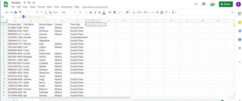
Please note: If your sheet name contains space characters, wrap the name in single quotation marks.

3. Google Sheets returns the value of the referenced cell. To copy the rest of the data, drag the small blue square at the bottom-right corner of the cell across the columns, then down the rows.

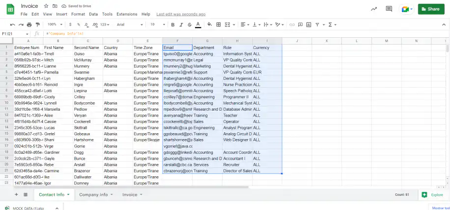
Note that this still requires manual input. As a result, it’s a method that’s only convenient if you don’t have a lot of data and would like to copy data within the same spreadsheet.

Copy a tab into another Google Sheets file

The following is another standard manual way to copy the tabs within the same spreadsheet or different ones.

1. Open the document containing the tabs you’d like to export. Right-click on the tab and select Copy to > Existing spreadsheet.

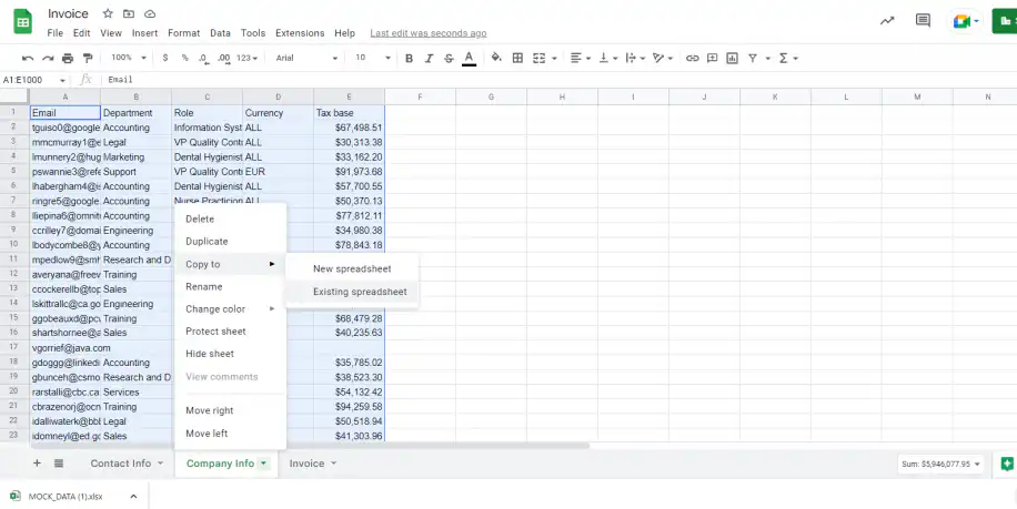
2. Select the file to which you’d like to copy the tab data. The file picker has three tabs: “My Drive”, “Shared with me”, and “Recent”. Click on the file and then press the “Select” blue button.

3. Once copied, you should get the confirmation message “Sheet copied successfully”. Press “OK” to continue or click on the link “Open spreadsheet”. The last option will open the destination file with the tab you just copied.

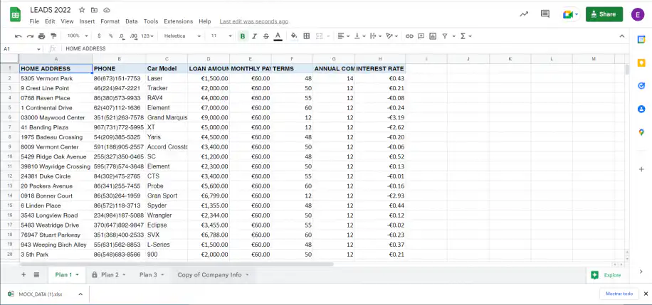
4. You should now see your tab appear in the destination spreadsheet. Here, “Copy of Company Info”.

How to combine data from multiple sheets with a formula

Although this method still involves some manual work, it’s more suitable for larger datasets. Here, you’ll learn how to combine data using two different formulas: IMPORTRANGE and QUERY.

Pull data from other files with IMPORTRANGE

IMPORTRANGE pulls a range from another Google Sheets file into the one you have open. Its syntax is =IMPORTRANGE("spreadsheet_url", "range_string"): the URL of the source file, then the tab and range to import, each in double quotation marks.

1. Open the file you want to pull data from and copy its URL from the address bar.

2. In the file that will hold the merged data, click an empty cell and enter the formula with that URL and the range, for example =IMPORTRANGE("URL of the source file", "Company Info!A1:E101"). Press Enter.

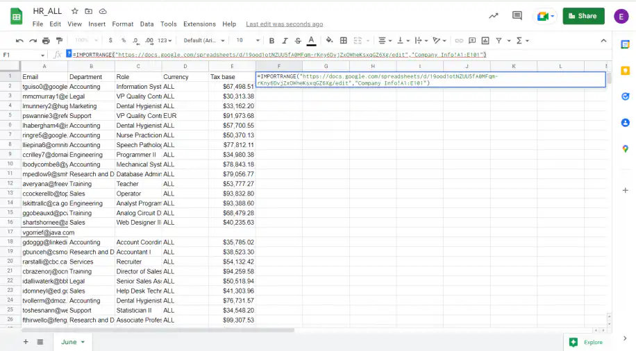
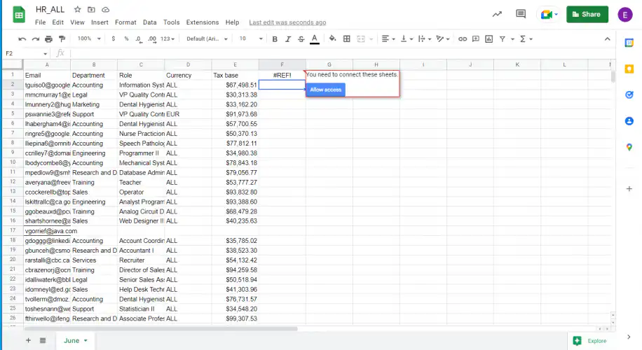
3. The first time you connect two files, the cell shows a #REF! error. Click the cell, then click Allow access.

4. The source data fills the cells to the right of and below the formula, here columns F to J.

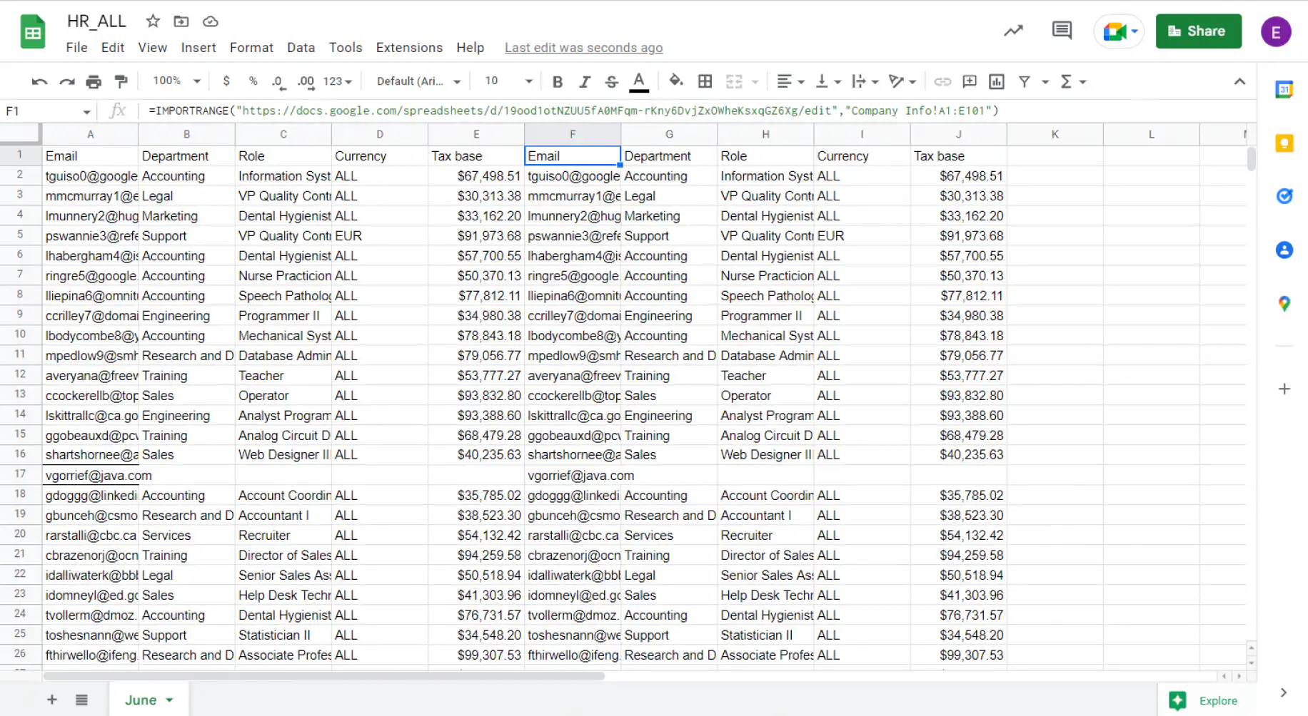
IMPORTRANGE brings in values only, without the source formatting, and large ranges take longer to load. When someone edits the source file, the imported data updates on its own. For more examples, see how to use IMPORTRANGE, or combine QUERY with IMPORTRANGE to filter the rows as they come in. To merge many files without formulas, try an IMPORTRANGE alternative.

Stack several tabs into one with QUERY

QUERY combines ranges from several tabs of the same file. Its syntax is =QUERY(data, query, headers). For data, put the ranges inside curly brackets. The query argument is a query string in double quotation marks, such as “select * where Col1 is not null”, which filters the combined rows. You can leave out query and headers to return every row, as in this example.

1. Click the first empty cell next to or below your data.

2. Type =QUERY, an opening parenthesis, and a curly bracket. Then enter each range as the tab name, an exclamation mark, and the cell range. Separate the ranges with a comma to place them side by side, or with a semicolon to stack them one under another. Close the bracket and the parenthesis. Here the formula is =QUERY({Sheet2!A1:E101,Sheet3!B1:C101}).

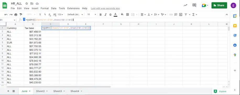
3. Press Enter. The two ranges appear side by side, starting in the formula cell.

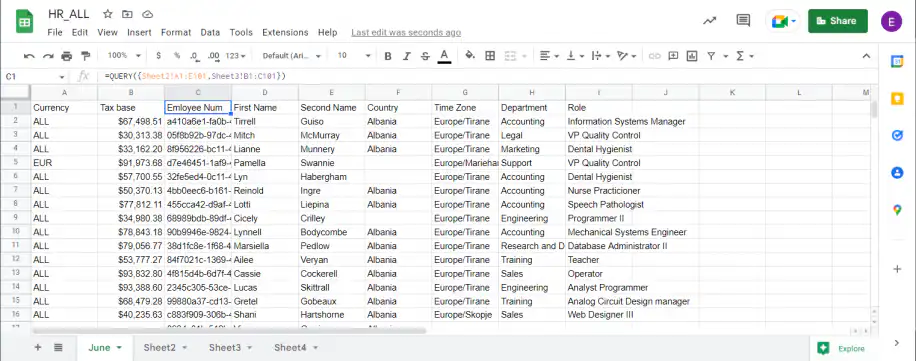
To stack tabs vertically, separate the ranges with semicolons, for example =QUERY({Sheet2!A2:E101;Sheet3!A2:E101}). Stacked ranges need the same number of columns, and ranges placed side by side need the same number of rows. If a tab name contains spaces, wrap it in single quotation marks, as in ‘Company Info’!A1:E101.

Data sharing in Google Sheets

While the shift to cloud-based software has made it easier to share data with colleagues, many of us still spend a lot of time gathering and collating information from different sheets and files.

There are many reasons for this.

Firstly, although online collaboration is great, you may not want to share the same spreadsheet with everyone on the team. If you’re a manager, you might need to collect data from colleagues’ personal files or multiple departments. Too many people working in one spreadsheet can be messy, and administrators often need to keep data separated for data protection reasons.

As well as data integrity and privacy issues, you don’t want one single file to become too large. Huge spreadsheets with multiple tabs are hard to navigate and easy to get lost in. Because it’s online software, the performance of Google Sheets may also be limited by your internet connection, and each file has a size limit of 5 million cells.

Combining data from multiple Google Sheets into one sheet can be tedious and time-consuming. Copy-pasting is a risky way to merge spreadsheets. As well as being slow, it’s prone to manual errors. ImportRange can work well inside one file, but if you’ve ever tried to use it to consolidate data from multiple Google Sheets files, you’ll know that it can generate errors.

Merge multiple Google Sheets into one automatically

A more reliable alternative to copy-pasting, ImportRange, or coding is Sheetgo: a no-code automation tool for spreadsheets. It lets you create connections between spreadsheets to push and pull data between different files and consolidate in Google Sheets.

This means you can combine data from different files and merge multiple Google Sheets into one automatically.

• Combine data from multiple Google Sheets into one file.
• Save time — no copy-pasting or manual work.
• Pull data from other Google Sheets into one central file.
• Consolidate Google Sheets data into reports and dashboards.
• Share team data without sharing the same spreadsheet
• Merge Google Sheets automatically with a system of interlinked spreadsheets.

How to combine Google Sheets files

In the following example, I’m going to show you how to consolidate data from three different Google Sheets files into one new spreadsheet.

Follow these steps to merge Google Sheets into one central file, to generate a summary sheet from multiple sources, or to pull Google Sheets data into a report or dashboard that updates automatically.

Step 1: Install Sheetgo

1. Open Sheetgo to start connecting your spreadsheets.
2. Login to Sheetgo with your Google, Microsoft, or Dropbox account.

Step 2: Start creating your Merge Google Sheets workflow

1. When you’ve logged in to the Sheetgo web app, click Create workflow. Then, select Connect files.
2. Give your workflow a name at the top of the screen so you can identify it later. Here I’ll call it Consolidate Google Sheets.
3. Under Select source data, choose Multiple files.

Step 3: Select the first file to merge

• Under Source data > Multiple files, select the first file you want to import data from.
• In the file box, click +Select file and select the file from your Google Drive.
• When the file appears on your Sheetgo screen, select the correct source tab (sheet).

In this example, I want to combine January delivery data from three company depots: North, South, and Central. Each warehouse logs daily dried fruit deliveries in their own Google Sheets file. I want to pull all of this data into one management spreadsheet that we use at central office.

To start with, I’ll select my first file: North depot deliveries, and the file tab January.

Step 4: Select further files to merge

When you’ve loaded the first file into Sheetgo, repeat the same process for the other files you want to merge data from.

Note that to consolidate correctly, every source tab (sheet) should have the same name and the same structure. This means that columns and headers should be the same in every spreadsheet.

• Click +Add another source file.
• Select an additional file and the correct source tab.
• Click Done.

Optional: identify source data origin

Before you continue with the connection, you have the option to configure the settings.

In this example, my three source files contain special formatting and data validation in the Date column. To import the dates correctly, I will activate the Transfer number formatting option.

• Click on Settings.
• Under Transfer formatting, enable Number formatting.

When you’re combining multiple Google Sheets files into one, it can be helpful to have the data origin clearly listed in the destination file.

• Click on Settings.
• Enable the Identify source feature.
• Under Identify source method, choose your desired identifier.

Sheetgo will add an extra column to your destination file, indicating where your source data came from. The source identifier can be the source location, the file name, the file creation date, or the file update date.

Here I want to see which depot the source data came from, so I’ll select File name as the identifier. The name of the source sheet will appear in a column next to the merged data.

Step 5: Choose where to merge the data

Now it’s time to select which Google Sheets file you want the data to be consolidated into.

You have the option to merge the data into a spreadsheet you’re already using, or a completely new Google Sheets file that Sheetgo will generate for you automatically. In both cases, Sheetgo will create a new tab(sheet) containing the merged data.

• Under Send data, click Google Sheets.
• Go to Destination > Google Sheets, then choose New file or Existing file.
• When sending data to a new file, give it a name in the File name box.
• If you want to save the file to a specific location in your Google Drive, click Change destination folder.
• Option: change the name of the file tab. If you leave this blank Sheetgo will automatically name the new destination tab Sheetgo_SourceTabName.

Here I’ll ask Sheetgo to create a new Google Sheets file for me automatically.

I’ll name the new file Total deliveries. In the new file tab box, I’ll call the tab All depots January. 

Step 6: Create the merge Google Sheets connection

• Click Finish and save to create the workflow.

Your destination file opens automatically inside Sheetgo.

As you can see, Sheetgo has created a new spreadsheet called Total deliveries with a tab called All depots January. This contains the merged data from my three source files.

Step 7: Update the workflow

Now that your Google Sheets files are connected, you can update the workflow at any time.

This will update each connection, pulling fresh data from the source sheets into the destination sheet. Any changes to the source files will be synced to the destination sheet.

To update the workflow manually,

• Open Sheetgo, select the workflow from your workflows list on the left of the screen.
• Click Run all automations at the bottom.

Step 8: Automate the workflow

To ensure that changes to the source files are regularly updated in the destination spreadsheet, schedule automatic updates. This means you don’t need to open a spreadsheet or open Sheetgo. Your data will flow automatically.

• Open your workflow and click Automate on the menu bar.
• Click Update automatically.
• Choose how often you want updates.
• Select the time of day and the day of the week.

How to combine Google Sheets in a folder

Sheetgo allows you to merge data from an unlimited amount of files into one central sheet.

If you want to merge a large number of Google Sheets, try consolidating from a folder. This is a quicker and more efficient way to combine data from multiple Google Sheets files.

On top of that, if you add a new file to the folder, it will be included in the next update automatically.

Instead of manually uploading every file you want to merge, just select one single Google Drive folder.

• Open Sheetgo and create a new workflow.
• Under Source Data, select Folder.

Just like when you upload files individually, it’s important to make sure that every source file has a source tab with the same name and structure.

How to manipulate merged data in Google Sheets

Once you’ve set up your data merging system, you’ll probably want to edit and process that data with formulas.

The Sheetgo-connected tab is dynamic, meaning that the data will be refreshed every time the workflow is updated.

To start working with the merged data, copy your imported data to another tab (sheet) using an array formula or a query. Need help? Learn more about queries here.

How to combine filtered data in Google Sheets

Here I’ve shown you how to import the entire source tab from each of the source files.

What if you only want to extract and combine specific Google Sheets data? That’s no problem: just apply a filter to the connection.

Let me return to my previous example to demonstrate.

This time, I only want to import delivery data on one item: Apricots.

• Open the workflow inside Sheetgo and go to Connections.
• On the right of the screen, go to the menu (⋮)
• Select Edit connection.

• Click on the Filter icon

Here I’ll use the condition option and the following settings:

• Data matches one condition (OR)
• Data matches > Condition > Column B : Category: Dried Fruit : Item.
• Criteria > Text is exactly.
• Value >Apricots.

When you’ve applied the conditions for your filter, click Finish and Save.

Here you can see that my Total deliveries file now only contains deliveries of apricots from my three warehouses.

Need more help exporting filtered data? Check out our in-depth guide on how to filter Google Sheets from one file to the other.

Which method to use

Cell references and copied tabs are enough for a one-off merge of a few tabs. IMPORTRANGE and QUERY handle larger ranges and other files, but someone has to fix the formulas when a tab or range changes. If you merge the same files every week, Sheetgo can run the merge on a schedule instead.

Sheetgo is an AI-powered data automation platform. A merged file that stays current is the step between scattered spreadsheets and data you can report on or hand to AI. Start a free trial and merge your first files.