Comment utiliser la fonction Excel VLOOKUP

Le VLOOKUP Excel function is undoubtedly one of the most useful functions that Excel offers. It can also be one of the most confusing functions if you aren’t familiar with it. In this article I’ll show you that the VLOOKUP function is actually quite simple, and how to use it to work with your spreadsheet data in all sorts of situations.

Essentially, the VLOOKUP Excel function searches for a value within a column, then returns a cell associated with that value (in the same row but a different column). This may sound confusing now, but I’ll show a few examples that will demonstrate how easy it really is!

Syntaxe

• valeur_de_recherche is the value you want the formula to search for
• table_array is the array that contains your data
• col_index_num tells the function which column to return a value from. For example, a value of 3 means the result will be from the third column of the table_array
• range_lookup is an optional parameter that can be either TRUE or FALSE. TRUE will provide an approximate match to the lookup_value while FALSE will mandate an exact match. The default is TRUE, but you’ll typically want to specify FALSE. I’ll talk more about this later

Comment utiliser la fonction Excel VLOOKUP

Alright, now that the technical stuff is out of the way, I’ll show you how to put this function to use. In the first example I’ll show the function in its most basic form. I have a list of data from a department store, and I want to input the employee in cell E2 and have the spreadsheet automatically tell me their sales in cell F2. I do that with the formula =VLOOKUP(E2,A2:C11,3,FALSE).

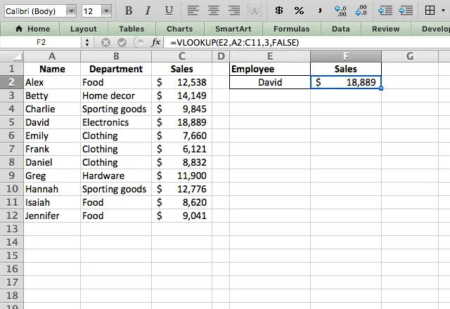
I’ll break this example down so you have a full understanding of it before moving on. My lookup_value here is a cell reference to cell E2, where I’ve typed the name “David”. I can type any of the employees’ names here and the formula will automatically adjust and tell me their sales number.

Next, I’ve selected the table_array of A2:C11. This array encompasses all my data. I then type 3 as my col_index_num which tells the function to return the answer from the third column of the array. With a quick look at the array you can see that the third column contains the sales information that I’m looking for.

Finally, I enter FALSE as my range_lookup because I want the function to find an exact match with my lookup_value. I’ll show the alternative to this in the next example.

So to recap what the function is doing: it’s taking my lookup_value (David) and searching for David in the first column of the table_array. When it finds David in row 5, it takes the value from the cell in row 5 and the third column in the array (which I instructed it to do when I typed 3).

Approximate match

That first example dealt with an exact match. But what happens when I specify TRUE as the range_lookup? I’ll demonstrate that here. For an approximate match, the function assumes that the data is sorted. It makes that assumption so that if it doesn’t find an exact match to the lookup_value, it can estimate what an approximate match would be.

In this example, I leave my data unsorted, which means that the approximate match won’t work properly. I’m doing this in order to demonstrate how it works, and then I’ll show how to use it properly.

La formule que j'utilise ici est la suivante =VLOOKUP(E2,A2:C12,3,TRUE). Note that it’s the exact same as in the previous example, except I typed TRUE instead of FALSE. Now what’s happening here? Remember, the function assumes that the data is sorted, so when it looks for Daniel it stops at David because in a sorted dataset, Daniel should be before David. Because of this, it returns the value prior to David (Emily’s sales) because that’s where Daniel should be.

In a sorted dataset, this might work alright. But when the data is not sorted, you can see that the answer here is completely wrong!

Approximate match (with sorted data)

OK, now that you understand how the function finds an approximate match, I’ll show how to do it correctly – with sorted data. In this example, I’m sorting the data by sales.

Note that I had to rearrange the columns because VLOOKUP can only search in the leftmost column.

The formula used here is =VLOOKUP(E2,A2:C12,2,TRUE). Even though nobody had exactly $15,000 in sales, the VLOOKUP Excel function correctly finds the closest value, and tells us who had it (Betty with $14,149).

Multiple lookup tables

You’ve now seen a few basic examples of the VLOOKUP Excel function in action. For the majority of Excel users, that’s all you really need to know.

But if you want to see what else the function can do, take a look at this example with multiple lookup tables.

In this example, the store pays out a bonus to employees based on their sales. However, the clothing department has a different bonus structure than the other employees. How can you use VLOOKUP to automatically give the correct bonus to each employee? I’ve done it here by typing =VLOOKUP(C2,IF(B2="Clothing",$F$3:$G$5,$F$9:$G$12),2,TRUE).

The trick here is that I have not one but two different tables that I want the function to search, depending on the situation. So I include an IF statement within the table_array parameter. The IF statement instructs the function to look in the Clothing table for employees in the clothing dept. and in the other bonus table for the other employees.

I added dollar signs ($) in the table_array because they tell Excel to hold those cells constant – so it doesn’t change the arrays when I drag the formula down from the first cell.

Pour découvrir d'autres façons de copier une formule vers le bas d'une colonne ou vers d'autres cellules, comme la poignée de recopie, le Collage spécial et les raccourcis clavier, consultez comment copier une formule dans Excel.

Two-way lookup

Now I’ll show you how to use VLOOKUP in a two-way lookup. In this example, I have sales numbers for both 2019 and 2020 for each employee.

I can use the MATCH function to get the numbers from the year I want, with the formula =VLOOKUP(G3,A2:D12,MATCH(G2,A1:D1,0),FALSE).

I put the MATCH function in the col_index_num parameter because I want the column that I get the results from to be variable.

Si votre table de recherche se trouve dans un autre onglet ou un autre fichier, découvrez comment utiliser VLOOKUP (RECHERCHEV) dans Excel depuis une autre feuille ou un autre classeur.

VLOOKUP Excel tips

• The VLOOKUP Excel function only looks to the right. So the column that you’re searching needs to be the leftmost column. If you need to search another column and can’t rearrange the data, you should check out how to use the combinaison INDEX MATCH.
• The VLOOKUP function returns the first match it finds. So if you have duplicated data in the search column, the function will return results for the first match it finds.
• The function is not case sensitive so don’t worry about upper- or lower-case letters causing mismatches.