This Google Sheets SWITCH evaluates an expression against a set of specific cases. The first case to evaluate as TRUE will return a corresponding value. If all cases are FALSE, the formula can return a default value.
The function works similarly to nested IF functions. But its syntax is much simpler, making it easy for anyone to read formulas in a spreadsheet.
It’s difficult to fully grasp this function without seeing some examples. But it’s worth the investment to learn how to use it.
Syntax
=SWITCH(logical_expression, case1, value1, [case2, value2]…, default)
- logical_expression– the expression to evaluate as TRUE or FALSE. This is what the function will test against each case.
- case1 – the first case to evaluate against the logical_expression.
- value1 – the value the function returns if case1 is TRUE.
- case2 – the second case to evaluate against the logical_expression.
- value2 –the value the function returns if case2 is TRUE.
- default– the value to return if all the cases are FALSE.
The logic behind this function is illustrated in the flowchart below.
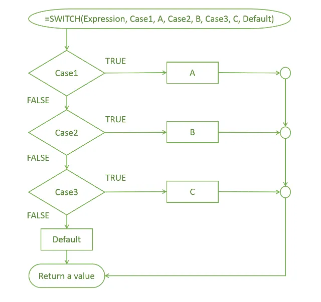
How to use the SWITCH function
Example 1: Basic use
Let’s start with the standard version of the function, and take a look at how it works.
=SWITCH(A2, 1, ”Alex”, 2, ”Bob”, 3, ”Charlie”, ”None”)

In this example, the expression is just ‘2’. It is compared with all three cases, and it matches the second case so the function returns the text ‘Bob’.
Example 2: Setting a default value
Let’s see what happens when none of the cases match the expression.
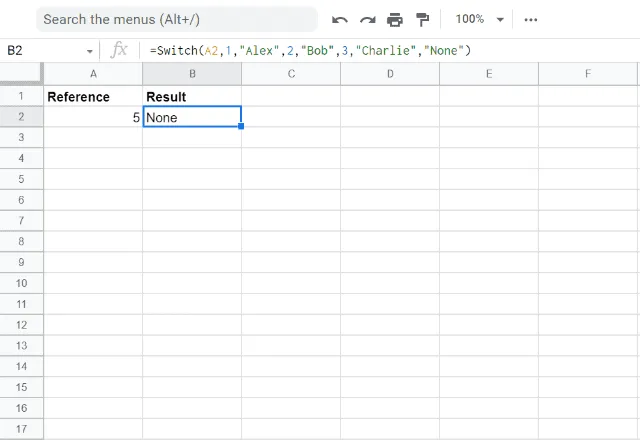
The expression ‘5’ is FALSE for all three cases, and as a result the function returns the default value ‘None’.
If you don’t define a default value the SWITCH function produces an error, as shown below.
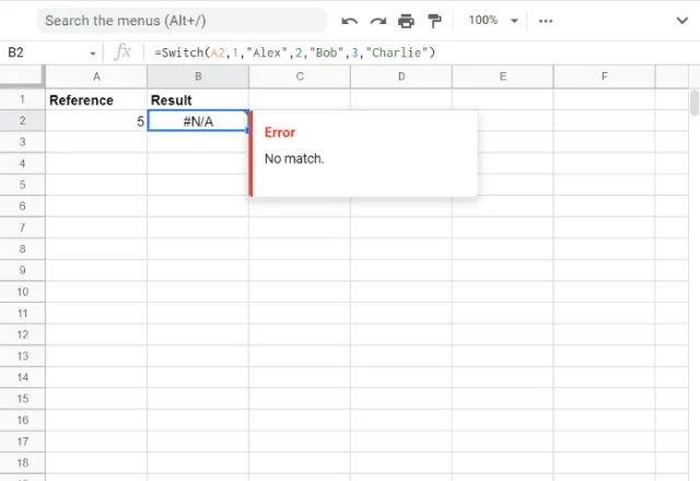
Example 3: Matching weekdays with colors
Say I’ve planned out my wardrobe for the week, with a different color for every weekday.
Column D has various weekdays and in column E SWITCH matches the day of the week with the correct color.
=SWITCH(C2, A2, B2, A3, B3, A4, B4, A5, B5, A6, B6, ”Not a valid weekday”)
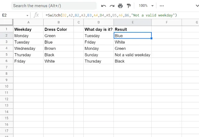
The function here is long, but you can easily break it down into three parts:
- The “What day is it?” column, basically what the function is looking for.
- After this, there are a series of case and value combinations. Each one declares that if the reference cell matches a weekday, then the function should output the corresponding color.
- Finally, there is a default value (“Not a valid weekday”) if none of the cases match the logical expression.
Should I use SWITCH or IF function?
The following example illustrates the benefits of the SWITCH function when compared to the IF function. It adapts the formula to use IF instead of SWITCH.
The formula is noticeably more complicated.
=IF(C2 = A2, B2, IF(C2 = A3, B3, IF(C2 = A4, B4, IF(C2 = A5, B5, IF(C2 = A6, B6, “Not a valid weekday”)))))

Use IF to perform logical tests on your data. As this function can be used with logical expressions such as “smaller than” or “greater than”.
Use SWITCH to work with exact matches within a dataset, as it will help avoid complex nested IF statements
Combining SWITCH with other functions
Using SWITCH with MONTH
Some date functions like MONTH return numbers that may be hard to interpret. You can use SWITCH to return more meaningful messages.
To replace the month numbers returned by MONTH you can set a case for each of the 12 potential results.
=SWITCH(MONTH(C21), 1, “JAN”, 2, “FEB”, 3, “MAR”, 4, “APR”, 5, “MAY”, 6, “JUN”, 7, “JUL”, 8, “AUG”, 9, “SEP”, 10, “OCT”, 11, “NOV”, 12, “DEC”, “No match”)
Using SWITCH with WEEKDAY
Similarly to MONTH, the output of WEEKDAY is difficult to read. Not only does it output numbers instead of text, the numbers can be set to correspond to different days.
This is the basic formula to use if Sunday is considered the first day of the week.
=SWITCH(WEEKDAY(C21, 1), 1, “SUN”, 2, “MON”, 3, “TUE”, 4, “WED”, 5, “THU”, 6, “FRI”, 7, “SAT”, “No match”)
Combining SWITCH with ERROR.TYPE
Another formula that returns cryptic codes is ERROR.TYPE, and SWITCH can replace them with more meaningful messages.
The formula below is just a starting point. It would be a good idea to adapt it to provide hints on how to fix these errors on your spreadsheet.
=IF(ISERROR(C21), SWITCH(ERROR.TYPE(C21), 1, “Null error”, 2, “Division by zero error”, 3, “Value error”, 4, “Reference error”, 5, “Name error”, 6, “Number error”, 7, “Not available error”, 8, “Getting data error”, 9, “Spill error”, 10, “Calc error”, “Unknown error”), “No error”)
Handle your data with Sheetgo
SWITCH is a great function, but it can only be used in a handful of cases. Sheetgo provides an arsenal of data processing tools to automate your workflows.
This platform has the potential to revolutionize your work, automating tedious tasks and sharing insights across your team.
These are just some of the key Sheetgo features:
- Automations – Link your data sources and schedule transfers to have your information available when you need it.
- Data processors – Query, merge and split data to suit your needs. Transfer data and keep its formatting.
- Sheetgo Forms – Create forms in seconds to conduct surveys and retrieve valuable information.
Try out Sheetgo today and start saving precious time.
SWITCH it up!
The SWITCH function in Google Sheets is an alternative to nested IF statements.
By evaluating an expression against a series of cases and returning the corresponding value for the first true case, it simplifies complex logical tests and makes your formulas easier to understand
Editor’s note: This is a revised version of a previous post that has been updated for accuracy and comprehensiveness.
