You are reading this post because you are probably tired of searching for duplicates in your Google Sheets. Finding these duplicates is like searching for a needle in a haystack, especially if there are 100+ rows.
In this article, we will share a quick way to highlight duplicates in Google Sheets, and share formulas and pro tips. Keep reading!
Key Takeaways:
- To highlight duplicates in Google Sheets, select the range > click Format > Conditional Formating > Format Rules > Custom Formula Is. Enter the formula =COUNTIF(A:A, A1) > 1 and click Done.
- =COUNTIF(A:A, A1)>1 is the formula to highlight duplicates in Google Sheets. Replace the letter A with the corresponding column.
- =COUNTIFS($B$1:$B,$B1,$C$1:$C,$C1) is the formula for highlighting duplicates in two columns. You can edit it to affect more columns.
How to Highlight Duplicates in Google Sheets? (2025 Tutorial)
How to Highlight Duplicates in Google Sheets
To highlight duplicates in Google Sheets, you need to set “Conditional Formatting” and use the formula “=COUNTIF(A:A, A1) > 1”.
Imagine you’re reviewing your inventory to identify the most popular products.
Your inventory list contains multiple entries for the same product, but they might be scattered throughout the sheet. Manually scanning the “Product Name” column would be inefficient and prone to errors, especially if your inventory is large.
Let’s see how to highlight duplicates using the formula mentioned above.
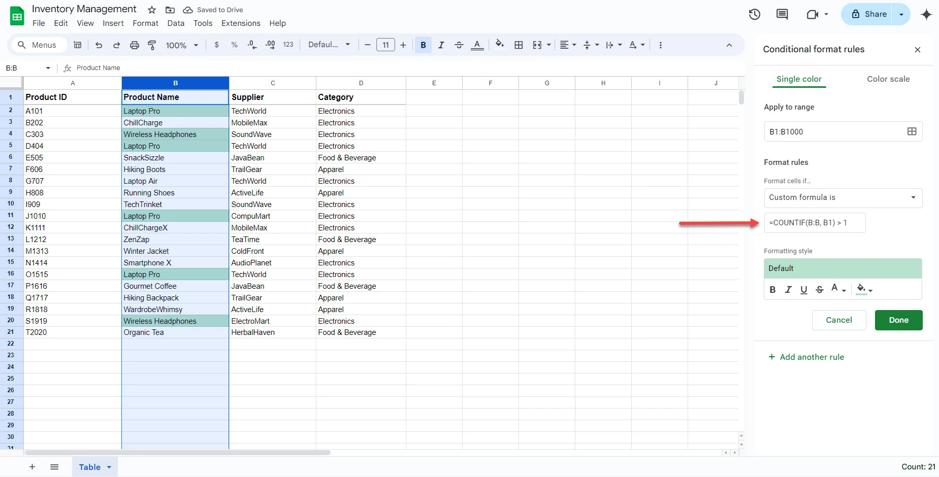
1. Select the entire “Product Name” column (Column B in our example).

2. Go to the “Format” menu and select “Conditional formatting.”

A sidebar will appear on the right.

3. In the sidebar, under “Format rules,” choose “Custom formula is.”

4. Enter the following formula in the text box: “=COUNTIF(B:B, B1) > 1” and click “Done.”

=COUNTIF(B:B, B1) looks at each cell in column B (Product Name). It then counts the number of times a product name appears in the whole column. > 1 means that if a product name appears more than once, it should be highlighted.
Our inventory example shows that “Laptop Pro” and “Wireless Headphones” appear more than once.
If you want to check column A, change the B in the formula to A. The new formula will be =COUNTIF(A:A, A1) > 1, and column C will be =COUNTIF(C:C, C1) > 1. Remember to select the matching range or column: A column for the A formula and C column for the C formula.

If you only want to highlight duplicates that appear more than ten times, change the number 1 to 10 at the end of the formula. The new formula will be: =COUNTIF(B:B, B1) > 10.
Want to learn more about formulas? Check our list of 100+ Google Sheets and Excel formulas.
The screenshot below shows a new scenario; “Laptop Pro” was highlighted because it appears more than ten times.

Check out our complete guide on how to use COUNTIF in Google Sheets.
How to Highlight Duplicates in Multiple Columns
Assume you want to know if you’ve bought a specific product from the same supplier more than once. This will help you identify your most frequent partners and negotiate better deals. In this case, you need to count the events where BOTH the “Product Name” AND the “Supplier” columns match.
So, let’s see how to highlight duplicates in multiple columns using “conditional formatting” and “absolute values.”
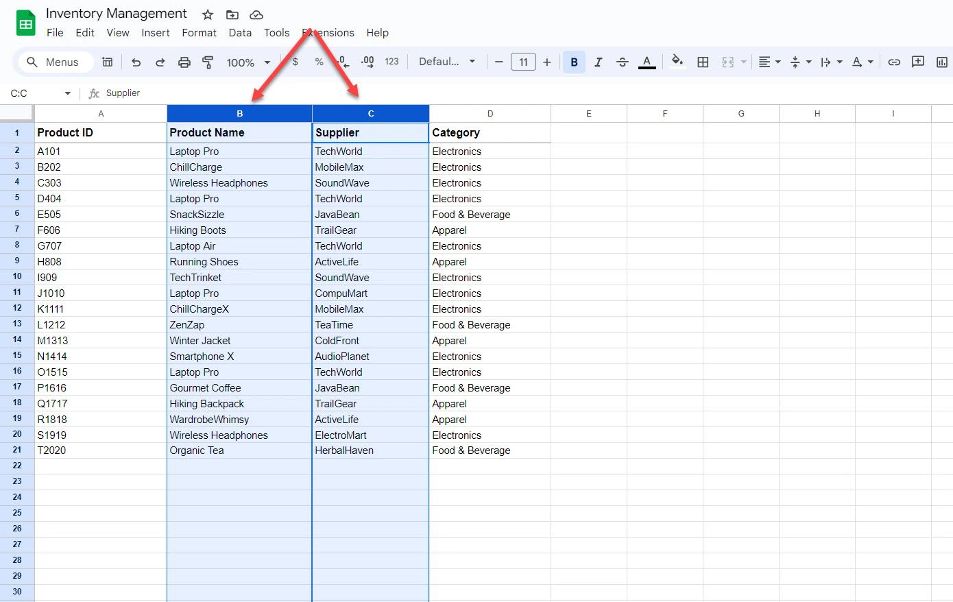
1. Select the entire table or the needed columns. In our case, we will select the “Product Name” and “Supplier” columns (columns B and C).

2. Go to the “Format” menu and select “Conditional formatting.”

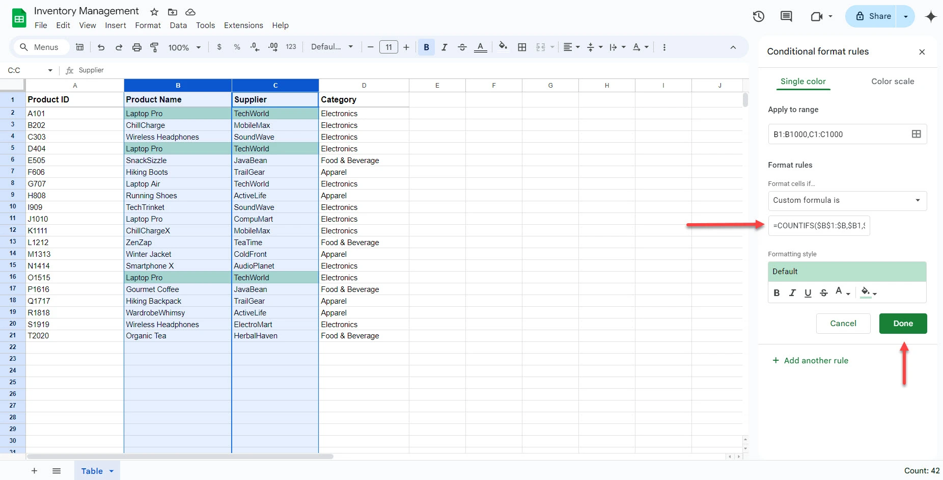
3. Under “Format rules,” choose “Custom formula is.”

4. Enter the following formula: =COUNTIFS($B$1:$B,$B1,$C$1:$C,$C1) > 1

=COUNTIFS($B$1:$B,$B1,$C$1:$C,$C1) looks at each cell in column B (Product Name) and column C (Supplier). It then counts the number of times columns B and C match. > 1 means B and C match more than once, it should be highlighted. The dollar signs ($) in the formula create absolute references. It ensures the formula works even when copied to other cells.
How to Remove Duplicates in Google Sheets?
Follow the steps below to remove duplicates in Google Sheets:
1. Select the range or entire sheet containing the data.

2. Go to Data > Data cleanup > Remove duplicates.

3. Choose whether your data has headers. In our case, we will check “Data has header now” since there is a header called “Product Name.”

4. Select the columns you want to check for duplicates.

5. Click “Remove duplicates.”

A popup will appear and indicate the number of rows removed.

The downside is this method removes entire rows, not individual cells.
Edit, Add, or Delete a Conditional Formatting Rule
Follow the steps below to edit, add, or delete a conditional formatting rule.
1. Select the range with the conditional formatting you want to edit.

2. Go to the “Format” menu and select “Conditional formatting.”

3. The sidebar will open and show the existing formatting rules for the selected range. Click on the rule you want to edit.

4. Update the format rules, formula, formatting style, or range as needed. Click “Done” to save the changes.

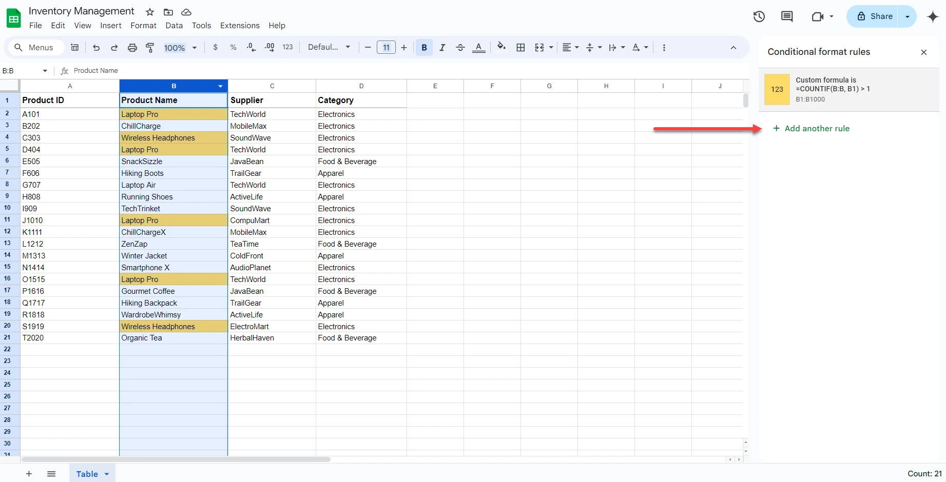
To add a new conditional formatting rule, follow steps 1-2 and click “Add another rule.”

To delete a conditional formatting rule, follow steps 1-2, hover your mouse over the rule, and click on the trash can icon next to it.

Rule Order Pro Tip:
If you have multiple rules for the same range, their order matters. Rules are evaluated from top to bottom, and the first rule that applies to a cell determines its formatting. You can reorder rules by clicking and dragging them in the sidebar.
If the formatting applied by a higher rule covers the conditions of a lower rule, the lower rule might be overridden or might not appear at all.
FAQ
Can I highlight duplicates in Google Sheets?
Yes, you can easily highlight duplicates in Google Sheets using conditional formatting.
What is the formula to highlight duplicates in Google Sheets?
The formula to highlight duplicates is: =COUNTIF(A:A, A1)>1. Use this formula if the range is A and change A to B if the range is B. You can use the formula in Conditional Formatting.

