At its core, countif is super simple: it counts every cell that meets a condition. Countif greater than 0 is just one of the many applications of this awesome function.
In this article we will see just how powerful this tool is and use it to the very limits of its capabilities. Even if you’ve used this function before you will surely find something new to try out.
Countif Syntax for Google Sheets
The structure for countif is as simple as it comes.
=COUNTIF(range, criterion)
- Range – cells for countif to test the criterion against.
- Criterion – test to apply to the range.
And that’s it, as simple as a function can get. But as we’ll explore there is more than meets the eye.
Different applications of countif
Let’s go over a handful of applications of this great function. Some of them include other functions, and others even have alternative functions with the same functionality.
Countif greater than 0
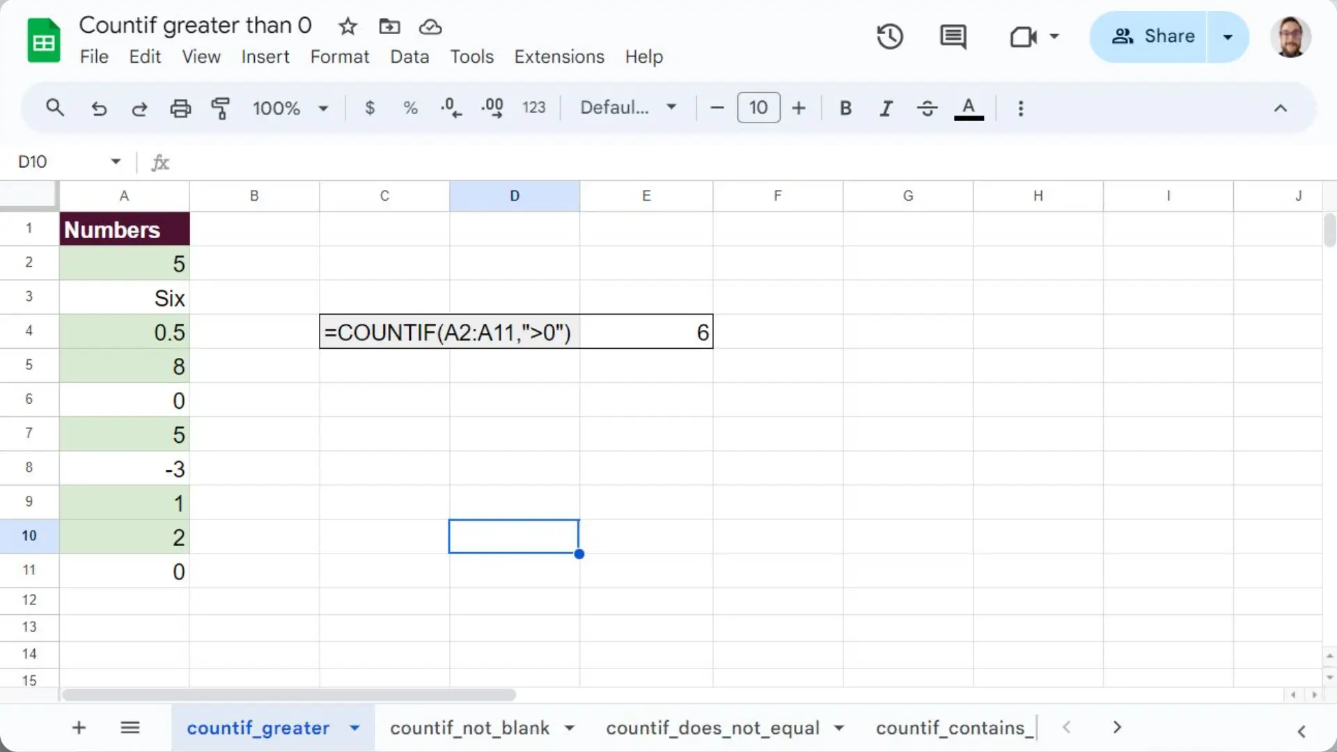
To count every number value over 0 all you have to do is use the greater than operator (“>”).
=COUNTIF(A2:A11,”>0″)
As you can see below, this won’t match exactly “0” or anything that isn’t a number.

Countif not blank
Here we will use the not equal to operator (“<>”) followed by nothing. This will count all cells that actually hold data. This can also be achieved with the counta function which is much simpler.
This formula is particularly useful when trying to assess how many data points are in a spreadsheet.
=COUNTIF(A2:A11,”<>”)
As expected this only counts 5 cells with data in the range.

Countif does not equal
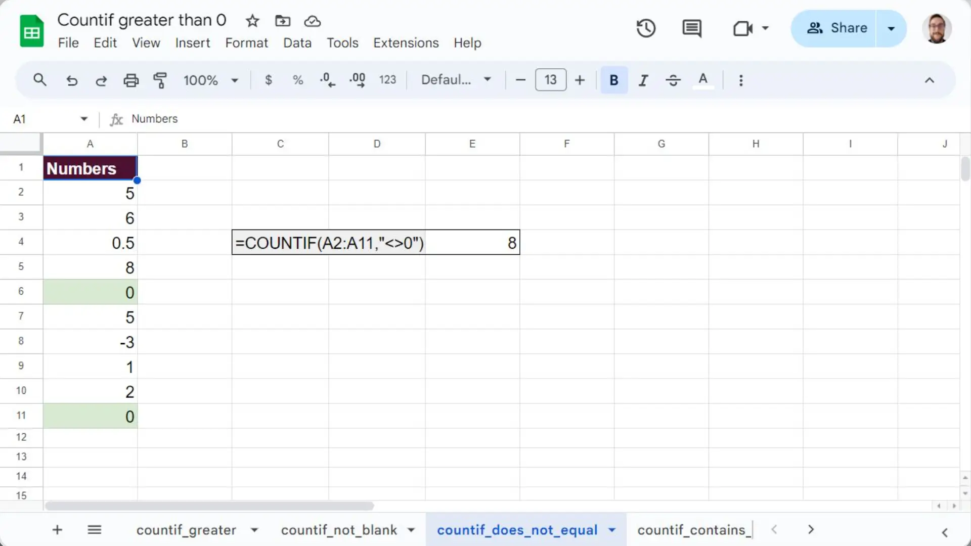
Just like in the previous example this can be achieved with the not equal to operator (“<>”). Only values other than the one specified will be counted.
=COUNTIF(A2:A11,”<>0″)
Using the same dataset in the count greater than 0 example, 8 cells were matched.

Countif contains partial text
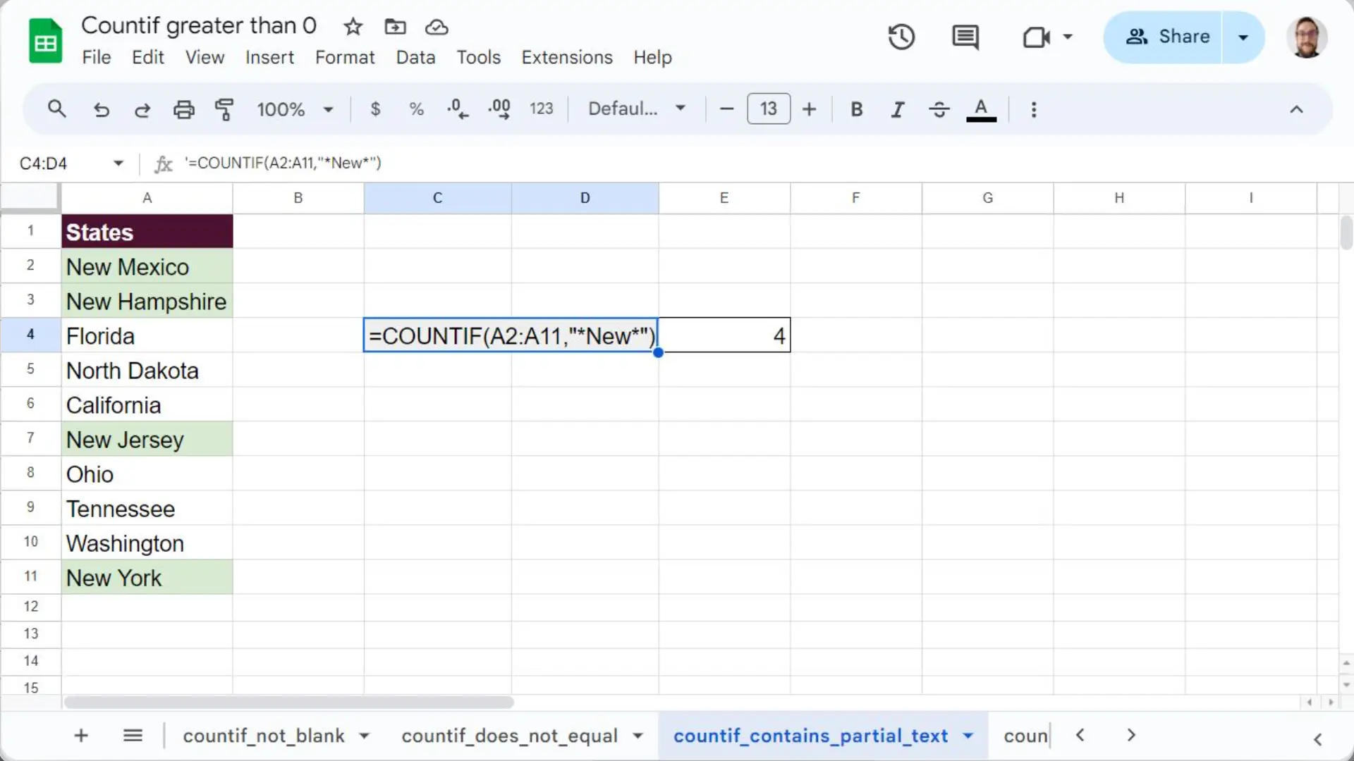
If you want to count cells with partial text matches, then you have to use the “*” wildcard. This will match any string values.
=COUNTIF(A2:A11,”*New*”)
In this example we matched only cells with the word “new” and counted states which include it in their name.

Countif month
This is where things start getting complex. This operation requires two new functions where the range would have been:
- MONTH – Extracts the month from a date and returns it as a number value. In this case we want to match 3 which is March.
- ARRAYFORMULA – Ensures that the MONTH function is applied to each cell in the range, rather than just the first cell.
=COUNTIF(ARRAYFORMULA(MONTH(A2:A11)), 3)
This formula matched 3 dates in the spreadsheet. Feel free to change the month function for its year or day counterparts to match different parts of a date. Make sure to also change the range and the expected value accordingly.

Google Sheets countif multiple criteria
Unfortunately, the only way to test against multiple criteria is to add the results from two separate countif functions. Clearly, this isn’t very elegant and you are much better off using countifs. Still it is worth trying this to remember that you can add the results of different functions.
=COUNTIF(A2:A11, “=5”) + COUNTIF(A2:A11, “=0”)

Get counting!
Now that you know various ways to count cells based on specific criteria you can count to your heart’s content. The countif formula is a great stepping stone on your spreadsheet journey.
Check out Sheetgo if you want to learn how you can connect spreadsheets and automate your business processes.

