Cómo utilizar la combinación de funciones INDEX MATCH de Excel

The INDEX and MATCH functions in Excel are both useful for a variety of purposes. But when you combine the two functions, they create an extremely powerful tool to search arrays of data and return their desired results. The INDEX and MATCH combination is essentially a more powerful and flexible version of the VLOOKUP function, which itself is a commonly used and handy function in Excel. In this article, I’ll demonstrate how to use the INDEX and MATCH combination, and show why it’s often better than the VLOOKUP function. But first, I’ll give an overview of the INDEX and MATCH functions individually.

Automatice las transferencias de datos más allá de Importrange

Descubra cómo

Función INDEX

El INDEX function in Excel returns the value of a cell specified by a certain number of column and row offsets. It works similar to the index of a book, which we use to quickly find certain content and chapters. To get an idea of how this works in practice, take a look at the example below.

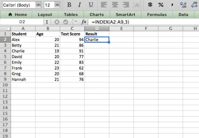
Here I’ve asked the INDEX function to give me the third value in the specified range. The function returns Charlie as the result, the third name in the list.

Función MATCH

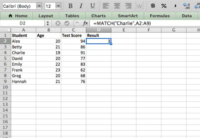
Now let’s take a look at the Función MATCH. This function does the exact opposite of the INDEX function – it takes a specified value and returns the location within an array.

Unlike the previous example, in which I asked the INDEX function to return the third name in the list, I now ask the MATCH function to find Charlie. As a result, the MATCH function tells me that Charlie is the third name in the list.

Now that I’ve highlighted both functions separately, I will demonstrate just how powerful they are when you use them together.

INDEX MATCH Excel function

Sintaxis

=INDEX(reference, MATCH(search_key, range, search_type), [MATCH(search_key, range, search_type)])

referencia – is the address of the range of cells within which the offset is evaluated from the very first cell (on the top left). Accordingly, the INDEX formula returns the value of the offset target cell.
buscar_clave - es el artículo que la función MATCH busca dentro del range de celdas. Puede ser un texto puro (‘Evan’), o una referencia de celda (como A7), or even a function that returns a string or a number (like LEFT(“Mike Johnson”,8) o DATE(2017,1,1)).
range – is the group of cells where the MATCH function searches for the item (search_key). This must be a one-dimensional array, i.e. either a range with a single column or a single row.
tipo_búsqueda - es una entrada opcional que indica cómo debe buscar la función MATCH el elemento buscar_clave en el range. This is typically 0, which indicates that it must be an exact MATCH.
You use the second MATCH function when searching a bi-dimensional array of data, for example if you need the MATCH function to identify both the vertical and horizontal offset.

Using the INDEX MATCH combination

The syntax above looks complicated, but I’ll give an example using the INDEX and MATCH combination in order to demonstrate how simple it really is.

Take a look at the screenshot below. I want the spreadsheet to tell me which person has a test score of 83. The formula I use for this example is =INDEX(A2:A9,MATCH(83,C2:C9,0)).

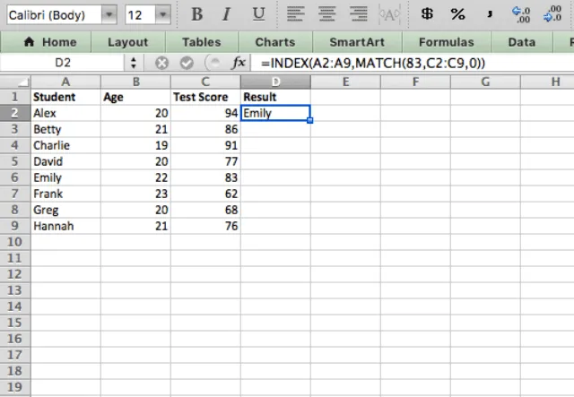
I’ve used the INDEX function, but instead of hardcoding the row number that I want it to return (like in the first example when I asked the INDEX function to return the third name of the list), I use the MATCH function to dynamically input the row that I want. The MATCH function takes my input (test score of 83) and tells the INDEX function in which row the number 83 appears. The INDEX function then takes that row number and selects the corresponding name (Emily).

At this point you might think “why don’t you just use the VLOOKUP function to do this?. Why bother combining two separate functions?” Well, there are a few different reasons, and they have to do with the limitations of the VLOOKUP function.

Limitations of the VLOOKUP function

The VLOOKUP function searches for a given input within an array, then outputs the data from another column corresponding to the row in which the input value was found. It is a very useful function, but it does have some limitations which I’ll outline below.

But first, here’s an example in which I use the VLOOKUP function to find the test score of Emily within the dataset.

Limitation 1 of VLOOKUP

The first limitation of the VLOOKUP function is that it can only be used to return the value in the leftmost column of the data. This wasn’t an issue in the previous example because there, I searched for the name of the student.

However, if I want to find the test score of Emily (by inputting “Emily” as the phrase to search for), the function returns an #N/A error. I asked to return a value (Test score) that is not in the leftmost column of the array.

Limitation 2 of VLOOKUP

The second limitation of the VLOOKUP function is that it is a static function that does not automatically update when you add new columns.

In the example below, I’ve used the same VLOOKUP function as in the previous example (finding the test score of Emily) and I’ve added a column to indicated whether or not each student lives on campus.

If the VLOOKUP function automatically updated, there would be no change to the result and I would still get Emily as the output. This is not the case however: the function returns 22 as the result.

This is obviously not the value I was searching for, and is a good example of how the VLOOKUP function won’t adapt to changes you make in your spreadsheet (like adding a new column for example).

If I do the same thing with an INDEX MATCH function on the other hand, the result doesn’t change.

Take a look at he example below. I’ve added an extra column to the data, and the INDEX MATCH function still works as a charm.

INDEX MATCH with two matches (Bi-dimensional array)

By now you’ve seen how useful the INDEX MATCH combination can be. But what if you have data that is 2-dimensional? In that case, you should use the INDEX function with two MATCH functions to get the value you’re looking for.

Here, you see a variety of test scores for different subjects of each student. The INDEX function combined with two MATCH functions identifies the test score for a specific student and a specific subject.

The function I use here is =INDEX(B2:F9,MATCH(B12,A2:A9,FALSE),MATCH(B13,B1:F1,FALSE)).

The logic behind this is the same as for a single INDEX MATCH combination: the MATCH function provides the “coordinates” of the desired value. This time, though, we need two MATCH functions: one to give the vertical offset, and one for the horizontal offset.

The best part is that I can type any student’s name and subject into cells B12 and B13 and immediately get the corresponding test score.